32.2 Una applicazione concreta
In questo tutorial esamineremo il modello di base LGM utilizzando un set di dati reali.
Considereremo il cambiamento nel rendimento in matematica dei bambini durante la scuola elementare e media utilizzando il set di dati NLSY-CYA (si veda Grimm, Ram, and Estabrook 2016). Iniziamo a leggere i dati.
# set filepath for data file
filepath <- "https://raw.githubusercontent.com/LRI-2/Data/main/GrowthModeling/nlsy_math_wide_R.dat"
# read in the text data file using the url() function
dat <- read.table(
file = url(filepath),
na.strings = "."
) # indicates the missing data designator
# copy data with new name
nlsy_math_wide <- dat
# Give the variable names
names(nlsy_math_wide) <- c(
"id", "female", "lb_wght", "anti_k1",
"math2", "math3", "math4", "math5", "math6", "math7", "math8",
"age2", "age3", "age4", "age5", "age6", "age7", "age8",
"men2", "men3", "men4", "men5", "men6", "men7", "men8",
"spring2", "spring3", "spring4", "spring5", "spring6", "spring7", "spring8",
"anti2", "anti3", "anti4", "anti5", "anti6", "anti7", "anti8"
)
# view the first few observations (and columns) in the data set
head(nlsy_math_wide[, 1:11], 10)
#> id female lb_wght anti_k1 math2 math3 math4 math5 math6 math7 math8
#> 1 201 1 0 0 NA 38 NA 55 NA NA NA
#> 2 303 1 0 1 26 NA NA 33 NA NA NA
#> 3 2702 0 0 0 56 NA 58 NA NA NA 80
#> 4 4303 1 0 0 NA 41 58 NA NA NA NA
#> 5 5002 0 0 4 NA NA 46 NA 54 NA 66
#> 6 5005 1 0 0 35 NA 50 NA 60 NA 59
#> 7 5701 0 0 2 NA 62 61 NA NA NA NA
#> 8 6102 0 0 0 NA NA 55 67 NA 81 NA
#> 9 6801 1 0 0 NA 54 NA 62 NA 66 NA
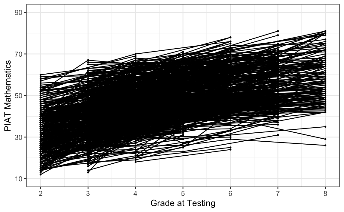
#> 10 6802 0 0 0 NA 55 NA 66 NA 68 NAIl nostro interesse specifico riguarda il cambiamento relativo alle misure ripetute di matematica, da math2 a math8.
Esaminiamo i dati.
# subsetting to variables of interest
nlsy_math_sub <- nlsy_math_wide[, c(
  "id", "math2", "math3", "math4",
  "math5", "math6", "math7", "math8"
)]
# reshaping wide to long
nlsy_math_long <- reshape(
  data = nlsy_math_sub,
  timevar = c("grade"),
  idvar = "id",
  varying = c(
    "math2", "math3", "math4",
    "math5", "math6", "math7", "math8"
  ),
  direction = "long", sep = ""
)
# sorting for easy viewing
# order by id and time
nlsy_math_long <- nlsy_math_long[order(nlsy_math_long$id, nlsy_math_long$grade), ]
# remove rows with NA for math (needed to get trajoctory lines connected)
nlsy_math_long <- nlsy_math_long[which(is.na(nlsy_math_long$math) == FALSE), ]

# intraindividual change trajetories
ggplot(
  data = nlsy_math_long, # data set
  aes(x = grade, y = math, group = id)
) + # setting variables
  geom_point(size = .5) + # adding points to plot
  geom_line() + # adding lines to plot
  theme_bw() + # changing style/background
  # setting the x-axis with breaks and labels
  scale_x_continuous(
    limits = c(2, 8),
    breaks = c(2, 3, 4, 5, 6, 7, 8),
    name = "Grade at Testing"
  ) +
  # setting the y-axis with limits breaks and labels
  scale_y_continuous(
    limits = c(10, 90),
    breaks = c(10, 30, 50, 70, 90),
    name = "PIAT Mathematics"
  )
References
Grimm, Kevin J, Nilam Ram, and Ryne Estabrook. 2016. Growth Modeling: Structural Equation and Multilevel Modeling Approaches. Guilford Publications.