32.4 Modello di crescita lineare
Nella discussione dei modelli di crescita, dopo il modello di assenza di crescita, si esamina sempre il modello di crescita lineare a causa della sua semplicità. Inoltre, i modelli di crescita lineare sono spesso un punto di partenza quando si cerca di comprendere il cambiamento all’interno della persona.
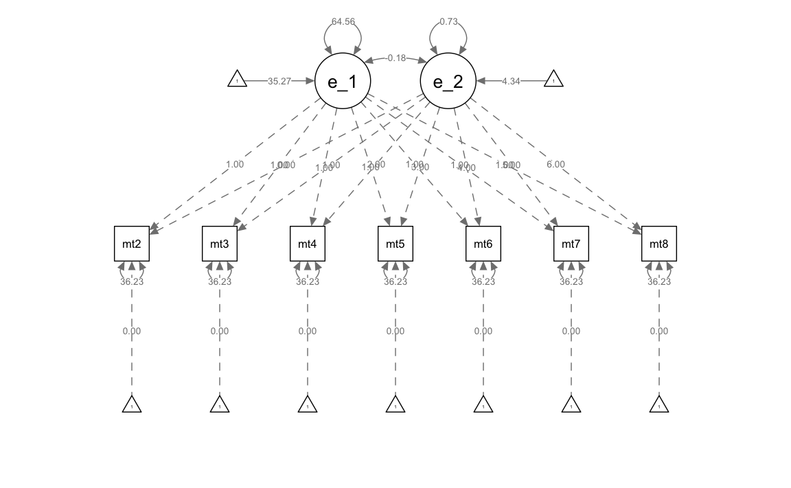
Implementiamo dunque un modello di crescita latente lineare.
lg_math_lavaan_model <- "
  # latent variable definitions
      #intercept (note intercept is a reserved term)
      eta_1 =~ 1*math2
      eta_1 =~ 1*math3
      eta_1 =~ 1*math4
      eta_1 =~ 1*math5
      eta_1 =~ 1*math6
      eta_1 =~ 1*math7
      eta_1 =~ 1*math8

      #linear slope
      eta_2 =~ 0*math2
      eta_2 =~ 1*math3
      eta_2 =~ 2*math4
      eta_2 =~ 3*math5
      eta_2 =~ 4*math6
      eta_2 =~ 5*math7
      eta_2 =~ 6*math8

  # factor variances
      eta_1 ~~ eta_1
      eta_2 ~~ eta_2

  # covariances among factors
      eta_1 ~~ eta_2

  # factor means
      eta_1 ~ start(35)*1
      eta_2 ~ start(4)*1

  # manifest variances (made equivalent by naming theta)
      math2 ~~ theta*math2
      math3 ~~ theta*math3
      math4 ~~ theta*math4
      math5 ~~ theta*math5
      math6 ~~ theta*math6
      math7 ~~ theta*math7
      math8 ~~ theta*math8
  # manifest means (fixed at zero)
      math2 ~ 0*1
      math3 ~ 0*1
      math4 ~ 0*1
      math5 ~ 0*1
      math6 ~ 0*1
      math7 ~ 0*1
      math8 ~ 0*1
" # end of model definition
Adattiamo il modello ai dati.
lg_math_lavaan_fit <- sem(lg_math_lavaan_model,
  data = nlsy_math_wide,
  meanstructure = TRUE,
  estimator = "ML",
  missing = "fiml"
)
Esaminiamo il risultato ottenuto.
summary(lg_math_lavaan_fit, fit.measures = TRUE)
#> lavaan 0.6.15 ended normally after 27 iterations
#>
#>   Estimator                                         ML
#>   Optimization method                           NLMINB
#>   Number of model parameters                        12
#>   Number of equality constraints                     6
#>
#>                                                   Used       Total
#>   Number of observations                           932         933
#>   Number of missing patterns                        60
#>
#> Model Test User Model:
#>
#>   Test statistic                               204.484
#>   Degrees of freedom                                29
#>   P-value (Chi-square)                           0.000
#>
#> Model Test Baseline Model:
#>
#>   Test statistic                               862.334
#>   Degrees of freedom                                21
#>   P-value                                        0.000
#>
#> User Model versus Baseline Model:
#>
#>   Comparative Fit Index (CFI)                    0.791
#>   Tucker-Lewis Index (TLI)                       0.849
#>
#>   Robust Comparative Fit Index (CFI)             0.896
#>   Robust Tucker-Lewis Index (TLI)                0.925
#>
#> Loglikelihood and Information Criteria:
#>
#>   Loglikelihood user model (H0)              -7968.693
#>   Loglikelihood unrestricted model (H1)      -7866.451
#>
#>   Akaike (AIC)                               15949.386
#>   Bayesian (BIC)                             15978.410
#>   Sample-size adjusted Bayesian (SABIC)      15959.354
#>
#> Root Mean Square Error of Approximation:
#>
#>   RMSEA                                          0.081
#>   90 Percent confidence interval - lower         0.070
#>   90 Percent confidence interval - upper         0.091
#>   P-value H_0: RMSEA <= 0.050                    0.000
#>   P-value H_0: RMSEA >= 0.080                    0.550
#>
#>   Robust RMSEA                                   0.134
#>   90 Percent confidence interval - lower         0.000
#>   90 Percent confidence interval - upper         0.233
#>   P-value H_0: Robust RMSEA <= 0.050             0.136
#>   P-value H_0: Robust RMSEA >= 0.080             0.792
#>
#> Standardized Root Mean Square Residual:
#>
#>   SRMR                                           0.121
#>
#> Parameter Estimates:
#>
#>   Standard errors                             Standard
#>   Information                                 Observed
#>   Observed information based on                Hessian
#>
#> Latent Variables:
#>                    Estimate  Std.Err  z-value  P(>|z|)
#>   eta_1 =~
#>     math2             1.000
#>     math3             1.000
#>     math4             1.000
#>     math5             1.000
#>     math6             1.000
#>     math7             1.000
#>     math8             1.000
#>   eta_2 =~
#>     math2             0.000
#>     math3             1.000
#>     math4             2.000
#>     math5             3.000
#>     math6             4.000
#>     math7             5.000
#>     math8             6.000
#>
#> Covariances:
#>                    Estimate  Std.Err  z-value  P(>|z|)
#>   eta_1 ~~
#>     eta_2            -0.181    1.150   -0.158    0.875
#>
#> Intercepts:
#>                    Estimate  Std.Err  z-value  P(>|z|)
#>     eta_1            35.267    0.355   99.229    0.000
#>     eta_2             4.339    0.088   49.136    0.000
#>    .math2             0.000
#>    .math3             0.000
#>    .math4             0.000
#>    .math5             0.000
#>    .math6             0.000
#>    .math7             0.000
#>    .math8             0.000
#>
#> Variances:
#>                    Estimate  Std.Err  z-value  P(>|z|)
#>     eta_1            64.562    5.659   11.408    0.000
#>     eta_2             0.733    0.327    2.238    0.025
#>    .math2   (thet)   36.230    1.867   19.410    0.000
#>    .math3   (thet)   36.230    1.867   19.410    0.000
#>    .math4   (thet)   36.230    1.867   19.410    0.000
#>    .math5   (thet)   36.230    1.867   19.410    0.000
#>    .math6   (thet)   36.230    1.867   19.410    0.000
#>    .math7   (thet)   36.230    1.867   19.410    0.000
#>    .math8   (thet)   36.230    1.867   19.410    0.000
Generiamo un diagramma di percorso.
Esaminiamo le traiettorie di crescita.
nlsy_math_predicted <- as.data.frame(cbind(nlsy_math_wide$id, lavPredict(lg_math_lavaan_fit)))

# naming columns
names(nlsy_math_predicted) <- c("id", "eta_1", "eta_2")

head(nlsy_math_predicted)
#>     id    eta_1    eta_2
#> 1  201 36.94675 4.534084
#> 2  303 26.03589 4.050780
#> 3 2702 49.70187 4.594148
#> 4 4303 41.04200 4.548063
#> 5 5002 37.01241 4.496745
#> 6 5005 37.68809 4.324197
# calculating implied manifest scores
nlsy_math_predicted$math2 <- 1 * nlsy_math_predicted$eta_1 + 0 * nlsy_math_predicted$eta_2
nlsy_math_predicted$math3 <- 1 * nlsy_math_predicted$eta_1 + 1 * nlsy_math_predicted$eta_2
nlsy_math_predicted$math4 <- 1 * nlsy_math_predicted$eta_1 + 2 * nlsy_math_predicted$eta_2
nlsy_math_predicted$math5 <- 1 * nlsy_math_predicted$eta_1 + 3 * nlsy_math_predicted$eta_2
nlsy_math_predicted$math6 <- 1 * nlsy_math_predicted$eta_1 + 4 * nlsy_math_predicted$eta_2
nlsy_math_predicted$math7 <- 1 * nlsy_math_predicted$eta_1 + 5 * nlsy_math_predicted$eta_2
nlsy_math_predicted$math8 <- 1 * nlsy_math_predicted$eta_1 + 6 * nlsy_math_predicted$eta_2
# reshaping wide to long
nlsy_math_predicted_long <- reshape(
data = nlsy_math_predicted,
timevar = c("grade"),
idvar = "id",
varying = c(
"math2", "math3", "math4",
"math5", "math6", "math7", "math8"
),
direction = "long", sep = ""
)
# sorting for easy viewing
# order by id and time
nlsy_math_predicted_long <- nlsy_math_predicted_long[order(nlsy_math_predicted_long$id, nlsy_math_predicted_long$grade), ]
# intraindividual change trajetories
ggplot(
data = nlsy_math_predicted_long[which(nlsy_math_predicted_long$id < 80000), ], # data set
aes(x = grade, y = math, group = id)
) + # setting variables
# geom_point(size=.5) + #adding points to plot
geom_line() + # adding lines to plot
theme_bw() + # changing style/background
# setting the x-axis with breaks and labels
scale_x_continuous(
limits = c(2, 8),
breaks = c(2, 3, 4, 5, 6, 7, 8),
name = "Grade at Testing"
) +
# setting the y-axis with limits breaks and labels
scale_y_continuous(
limits = c(10, 90),
breaks = c(10, 30, 50, 70, 90),
name = "Predicted PIAT Mathematics"
)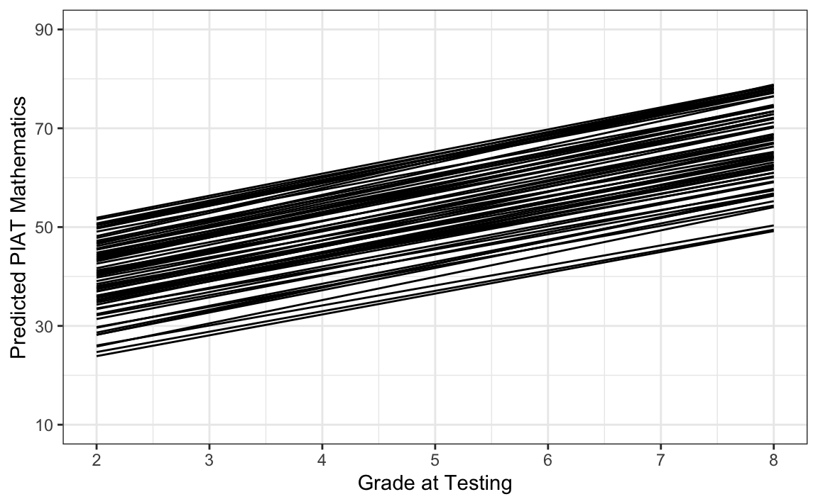
Dal grafico si può notare che questo modello rappresenta la traiettoria di ogni bambino come una linea retta, con alcune differenze interindividuali nella velocità del cambiamento intraindividuale. Questo tutorial ha dunque illustrato come impostare e adattare modelli di crescita lineare nel framework di modellizzazione SEM utilizzando il pacchetto lavaan in R, nonché come calcolare e rappresentare graficamente le traiettorie di crescita previste dal modello.