Capitolo 34 Covariate indipendenti dal tempo
Partendo dai modelli di crescita lineare descritti nei capitoli precedenti, ci chiediamo se le differenze individuali nelle traiettorie di cambiamento siano associate ad altre variabili. Questo capitolo introduce modelli che esaminano se la variabilità nell’intercetta e nella pendenza del modello di crescita lineare può essere spiegata da covariate invarianti nel tempo. Queste sono variabili a livello di persona che non cambiano nel tempo, come il genere, le condizioni sperimentali e lo stato socio-economico. Nel contesto dei modelli a crescita latente, tali variabili vengono considerate come variabili indipendenti in un modello di regressione multipla in cui l’intercetta e la pendenza del modello di crescita lineare sono le variabili dipendenti. Le covariate invarianti nel tempo possono essere continue, ordinali o categoriche.
Studiando come le differenze individuali nell’intercetta e nella pendenza sono correlate ad altre variabili a livello della persona, possiamo comprendere le possibili ragioni per cui gli individui cambiano in modi diversi. Tuttavia, i risultati di questi modelli non forniscono ulteriori inferenze sulla causalità rispetto ai tipici modelli di regressione. Gli utenti dovrebbero essere cauti quando discutono tali effetti e tenere presente se la covariata invariante nel tempo è stata assegnata in maniera casuale nel contesto di un protocollo sperimentale, oppure se i dati provengono da ricerche osservazionali.
Per questo esempio considereremo i dati di prestazione matematica dal data set NLSY-CYA Long Data (si veda Grimm, Ram, and Estabrook 2016). Iniziamo a leggere i dati.
# set filepath for data file
filepath <- "https://raw.githubusercontent.com/LRI-2/Data/main/GrowthModeling/nlsy_math_long_R.dat"
# read in the text data file using the url() function
dat <- read.table(
file = url(filepath),
na.strings = "."
) # indicates the missing data designator
# copy data with new name
nlsy_math_long <- dat
# Add names the columns of the data set
names(nlsy_math_long) <- c(
"id", "female", "lb_wght",
"anti_k1", "math", "grade",
"occ", "age", "men",
"spring", "anti"
)
# view the first few observations in the data set
head(nlsy_math_long, 10)
#> id female lb_wght anti_k1 math grade occ age men spring anti
#> 1 201 1 0 0 38 3 2 111 0 1 0
#> 2 201 1 0 0 55 5 3 135 1 1 0
#> 3 303 1 0 1 26 2 2 121 0 1 2
#> 4 303 1 0 1 33 5 3 145 0 1 2
#> 5 2702 0 0 0 56 2 2 100 NA 1 0
#> 6 2702 0 0 0 58 4 3 125 NA 1 2
#> 7 2702 0 0 0 80 8 4 173 NA 1 2
#> 8 4303 1 0 0 41 3 2 115 0 0 1
#> 9 4303 1 0 0 58 4 3 135 0 1 2
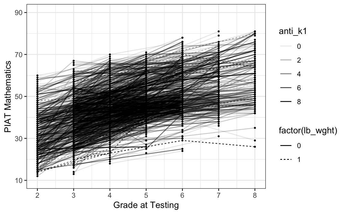
#> 10 5002 0 0 4 46 4 2 117 NA 1 4# intraindividual change trajetories
ggplot(
data = nlsy_math_long, # data set
aes(x = grade, y = math, group = id)
) + # setting variables
geom_point(size = .5) + # adding points to plot
geom_line(aes(linetype = factor(lb_wght), alpha = anti_k1)) + # adding lines to plot
theme_bw() + # changing style/background
# setting the x-axis with breaks and labels
scale_x_continuous(
limits = c(2, 8),
breaks = c(2, 3, 4, 5, 6, 7, 8),
name = "Grade at Testing"
) +
# setting the y-axis with limits breaks and labels
scale_y_continuous(
limits = c(10, 90),
breaks = c(10, 30, 50, 70, 90),
name = "PIAT Mathematics"
)
Per semplicità, leggiamo gli stessi dati in formato wide da un file.
# set filepath for data file
filepath <- "https://raw.githubusercontent.com/LRI-2/Data/main/GrowthModeling/nlsy_math_wide_R.dat"
# read in the text data file using the url() function
dat <- read.table(
file = url(filepath),
na.strings = "."
) # indicates the missing data designator
# copy data with new name
nlsy_math_wide <- dat
# Give the variable names
names(nlsy_math_wide) <- c(
"id", "female", "lb_wght", "anti_k1",
"math2", "math3", "math4", "math5", "math6", "math7", "math8",
"age2", "age3", "age4", "age5", "age6", "age7", "age8",
"men2", "men3", "men4", "men5", "men6", "men7", "men8",
"spring2", "spring3", "spring4", "spring5", "spring6", "spring7", "spring8",
"anti2", "anti3", "anti4", "anti5", "anti6", "anti7", "anti8"
)
# view the first few observations (and columns) in the data set
head(nlsy_math_wide[, 1:11], 10)
#> id female lb_wght anti_k1 math2 math3 math4 math5 math6 math7 math8
#> 1 201 1 0 0 NA 38 NA 55 NA NA NA
#> 2 303 1 0 1 26 NA NA 33 NA NA NA
#> 3 2702 0 0 0 56 NA 58 NA NA NA 80
#> 4 4303 1 0 0 NA 41 58 NA NA NA NA
#> 5 5002 0 0 4 NA NA 46 NA 54 NA 66
#> 6 5005 1 0 0 35 NA 50 NA 60 NA 59
#> 7 5701 0 0 2 NA 62 61 NA NA NA NA
#> 8 6102 0 0 0 NA NA 55 67 NA 81 NA
#> 9 6801 1 0 0 NA 54 NA 62 NA 66 NA
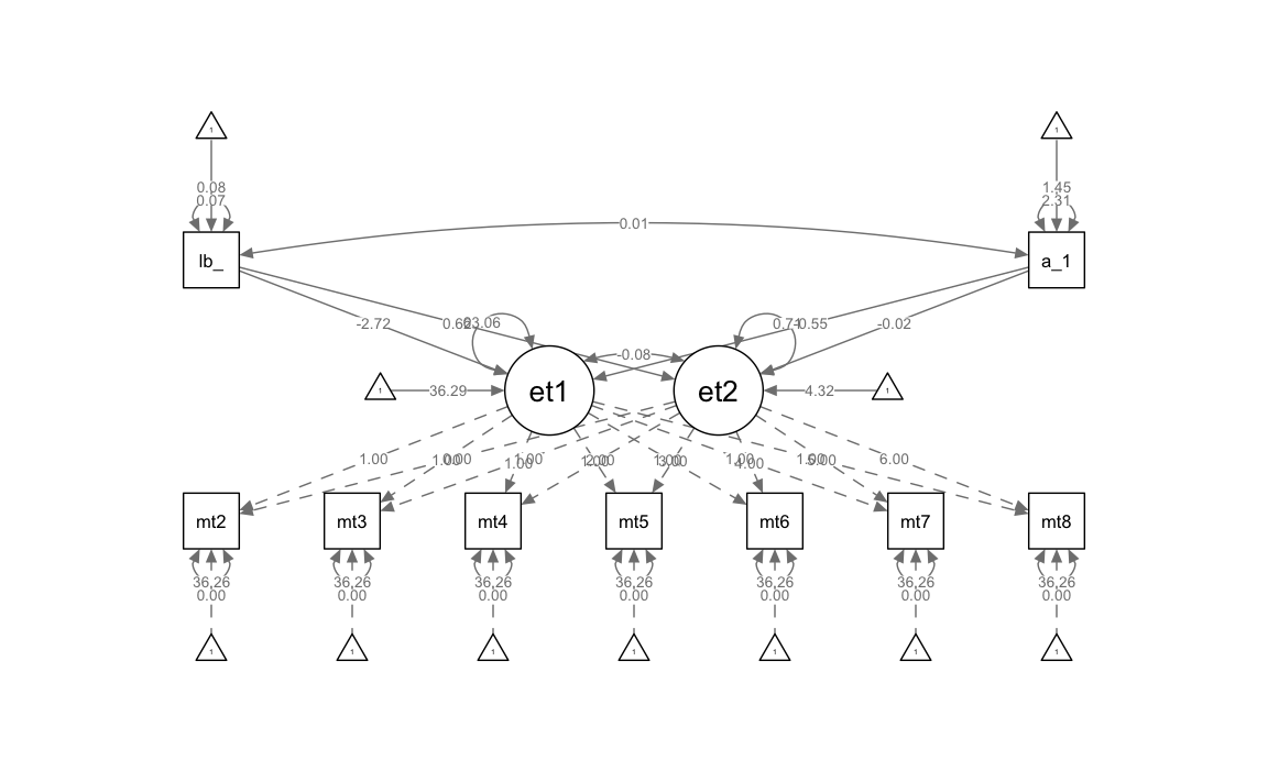
#> 10 6802 0 0 0 NA 55 NA 66 NA 68 NASpecifichiamo il modello SEM.
# writing out linear growth model with tic in full SEM way
lg_math_tic_lavaan_model <- "
    #latent variable definitions
            #intercept
              eta1 =~ 1*math2+
                      1*math3+
                      1*math4+
                      1*math5+
                      1*math6+
                      1*math7+
                      1*math8
            #linear slope
              eta2 =~ 0*math2+
                      1*math3+
                      2*math4+
                      3*math5+
                      4*math6+
                      5*math7+
                      6*math8

          #factor variances
            eta1 ~~ eta1
            eta2 ~~ eta2

          #factor covariance
            eta1 ~~ eta2

          #manifest variances (set equal by naming theta)
            math2 ~~ theta*math2
            math3 ~~ theta*math3
            math4 ~~ theta*math4
            math5 ~~ theta*math5
            math6 ~~ theta*math6
            math7 ~~ theta*math7
            math8 ~~ theta*math8

          #latent means (freely estimated)
            eta1 ~ 1
            eta2 ~ 1

          #manifest means (fixed to zero)
            math2 ~ 0*1
            math3 ~ 0*1
            math4 ~ 0*1
            math5 ~ 0*1
            math6 ~ 0*1
            math7 ~ 0*1
            math8 ~ 0*1

        #Time invariant covaraite
          #regression of time-invariant covariate on intercept and slope factors
            eta1~lb_wght+anti_k1
            eta2~lb_wght+anti_k1

        #variance of TIV covariates
            lb_wght ~~ lb_wght
            anti_k1 ~~ anti_k1

        #covariance of TIV covaraites
            lb_wght ~~ anti_k1

        #means of TIV covariates (freely estimated)
            lb_wght ~ 1
            anti_k1 ~ 1
" # end of model definition
Adattiamo il modello ai dati.
lg_math_tic_lavaan_fit <- sem(lg_math_tic_lavaan_model,
  data = nlsy_math_wide,
  meanstructure = TRUE,
  estimator = "ML",
  missing = "fiml"
)
Esaminiamo la soluzione ottenuta.
summary(lg_math_tic_lavaan_fit, fit.measures = TRUE)
#> lavaan 0.6.15 ended normally after 117 iterations
#>
#>   Estimator                                         ML
#>   Optimization method                           NLMINB
#>   Number of model parameters                        21
#>   Number of equality constraints                     6
#>
#>   Number of observations                           933
#>   Number of missing patterns                        61
#>
#> Model Test User Model:
#>
#>   Test statistic                               220.221
#>   Degrees of freedom                                39
#>   P-value (Chi-square)                           0.000
#>
#> Model Test Baseline Model:
#>
#>   Test statistic                               892.616
#>   Degrees of freedom                                36
#>   P-value                                        0.000
#>
#> User Model versus Baseline Model:
#>
#>   Comparative Fit Index (CFI)                    0.788
#>   Tucker-Lewis Index (TLI)                       0.805
#>
#>   Robust Comparative Fit Index (CFI)             0.920
#>   Robust Tucker-Lewis Index (TLI)                0.926
#>
#> Loglikelihood and Information Criteria:
#>
#>   Loglikelihood user model (H0)              -9785.085
#>   Loglikelihood unrestricted model (H1)      -9674.975
#>
#>   Akaike (AIC)                               19600.171
#>   Bayesian (BIC)                             19672.747
#>   Sample-size adjusted Bayesian (SABIC)      19625.108
#>
#> Root Mean Square Error of Approximation:
#>
#>   RMSEA                                          0.071
#>   90 Percent confidence interval - lower         0.062
#>   90 Percent confidence interval - upper         0.080
#>   P-value H_0: RMSEA <= 0.050                    0.000
#>   P-value H_0: RMSEA >= 0.080                    0.046
#>
#>   Robust RMSEA                                   0.100
#>   90 Percent confidence interval - lower         0.000
#>   90 Percent confidence interval - upper         0.183
#>   P-value H_0: Robust RMSEA <= 0.050             0.218
#>   P-value H_0: Robust RMSEA >= 0.080             0.654
#>
#> Standardized Root Mean Square Residual:
#>
#>   SRMR                                           0.097
#>
#> Parameter Estimates:
#>
#>   Standard errors                             Standard
#>   Information                                 Observed
#>   Observed information based on                Hessian
#>
#> Latent Variables:
#>                    Estimate  Std.Err  z-value  P(>|z|)
#>   eta1 =~
#>     math2             1.000
#>     math3             1.000
#>     math4             1.000
#>     math5             1.000
#>     math6             1.000
#>     math7             1.000
#>     math8             1.000
#>   eta2 =~
#>     math2             0.000
#>     math3             1.000
#>     math4             2.000
#>     math5             3.000
#>     math6             4.000
#>     math7             5.000
#>     math8             6.000
#>
#> Regressions:
#>                    Estimate  Std.Err  z-value  P(>|z|)
#>   eta1 ~
#>     lb_wght          -2.716    1.294   -2.099    0.036
#>     anti_k1          -0.551    0.232   -2.369    0.018
#>   eta2 ~
#>     lb_wght           0.625    0.333    1.873    0.061
#>     anti_k1          -0.019    0.059   -0.327    0.743
#>
#> Covariances:
#>                    Estimate  Std.Err  z-value  P(>|z|)
#>  .eta1 ~~
#>    .eta2             -0.078    1.145   -0.068    0.945
#>   lb_wght ~~
#>     anti_k1           0.007    0.014    0.548    0.584
#>
#> Intercepts:
#>                    Estimate  Std.Err  z-value  P(>|z|)
#>    .eta1             36.290    0.497   73.052    0.000
#>    .eta2              4.315    0.122   35.420    0.000
#>    .math2             0.000
#>    .math3             0.000
#>    .math4             0.000
#>    .math5             0.000
#>    .math6             0.000
#>    .math7             0.000
#>    .math8             0.000
#>     lb_wght           0.080    0.009    9.031    0.000
#>     anti_k1           1.454    0.050   29.216    0.000
#>
#> Variances:
#>                    Estimate  Std.Err  z-value  P(>|z|)
#>    .eta1             63.064    5.609   11.242    0.000
#>    .eta2              0.713    0.326    2.185    0.029
#>    .math2   (thet)   36.257    1.868   19.406    0.000
#>    .math3   (thet)   36.257    1.868   19.406    0.000
#>    .math4   (thet)   36.257    1.868   19.406    0.000
#>    .math5   (thet)   36.257    1.868   19.406    0.000
#>    .math6   (thet)   36.257    1.868   19.406    0.000
#>    .math7   (thet)   36.257    1.868   19.406    0.000
#>    .math8   (thet)   36.257    1.868   19.406    0.000
#>     lb_wght           0.074    0.003   21.599    0.000
#>     anti_k1           2.312    0.107   21.599    0.000
Creiamo un diagramma di percorso.
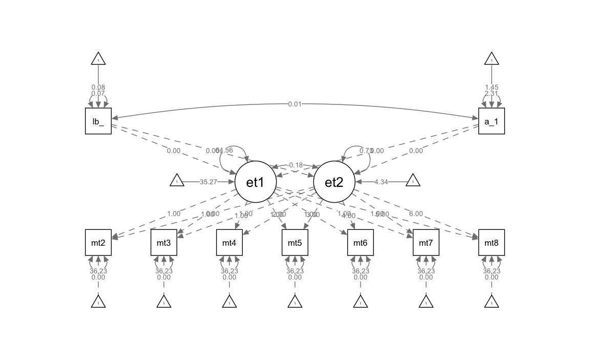
34.0.1 Valutare il contributo delle covariate
Per valutare se le covariate considerate forniscono un contributo sostanziale al modello confronteremo il modello precedente con un modello vincolato in cui l’effetto delle covariate viene fissato come uguale a zero.
# writing out linear growth model with tic in full SEM way
lg_math_ticZERO_lavaan_model <- "
    #latent variable definitions
            #intercept
              eta1 =~ 1*math2+
                      1*math3+
                      1*math4+
                      1*math5+
                      1*math6+
                      1*math7+
                      1*math8
            #linear slope
              eta2 =~ 0*math2+
                      1*math3+
                      2*math4+
                      3*math5+
                      4*math6+
                      5*math7+
                      6*math8

          #factor variances
            eta1 ~~ eta1
            eta2 ~~ eta2

          #factor covariance
            eta1 ~~ eta2

          #manifest variances (set equal by naming theta)
            math2 ~~ theta*math2
            math3 ~~ theta*math3
            math4 ~~ theta*math4
            math5 ~~ theta*math5
            math6 ~~ theta*math6
            math7 ~~ theta*math7
            math8 ~~ theta*math8

          #latent means (freely estimated)
            eta1 ~ 1
            eta2 ~ 1

          #manifest means (fixed to zero)
            math2 ~ 0*1
            math3 ~ 0*1
            math4 ~ 0*1
            math5 ~ 0*1
            math6 ~ 0*1
            math7 ~ 0*1
            math8 ~ 0*1

        #Time invariant covaraite
          #regression of time-invariant covariate on intercept and slope factors
          #FIXED to 0
            eta1~0*lb_wght+0*anti_k1
            eta2~0*lb_wght+0*anti_k1

        #variance of TIV covariates
            lb_wght ~~ lb_wght
            anti_k1 ~~ anti_k1

        #covariance of TIV covaraites
            lb_wght ~~ anti_k1

        #means of TIV covariates (freely estimated)
            lb_wght ~ 1
            anti_k1 ~ 1
" # end of model definition
Adattiamo il modello ai dati.
lg_math_ticZERO_lavaan_fit <- sem(lg_math_ticZERO_lavaan_model,
  data = nlsy_math_wide,
  meanstructure = TRUE,
  estimator = "ML",
  missing = "fiml"
)
Esaminiamo il risultato ottenuto.
summary(lg_math_ticZERO_lavaan_fit, fit.measures = TRUE)
#> lavaan 0.6.15 ended normally after 102 iterations
#>
#>   Estimator                                         ML
#>   Optimization method                           NLMINB
#>   Number of model parameters                        17
#>   Number of equality constraints                     6
#>
#>   Number of observations                           933
#>   Number of missing patterns                        61
#>
#> Model Test User Model:
#>
#>   Test statistic                               234.467
#>   Degrees of freedom                                43
#>   P-value (Chi-square)                           0.000
#>
#> Model Test Baseline Model:
#>
#>   Test statistic                               892.616
#>   Degrees of freedom                                36
#>   P-value                                        0.000
#>
#> User Model versus Baseline Model:
#>
#>   Comparative Fit Index (CFI)                    0.776
#>   Tucker-Lewis Index (TLI)                       0.813
#>
#>   Robust Comparative Fit Index (CFI)             0.917
#>   Robust Tucker-Lewis Index (TLI)                0.931
#>
#> Loglikelihood and Information Criteria:
#>
#>   Loglikelihood user model (H0)              -9792.208
#>   Loglikelihood unrestricted model (H1)      -9674.975
#>
#>   Akaike (AIC)                               19606.416
#>   Bayesian (BIC)                             19659.638
#>   Sample-size adjusted Bayesian (SABIC)      19624.703
#>
#> Root Mean Square Error of Approximation:
#>
#>   RMSEA                                          0.069
#>   90 Percent confidence interval - lower         0.061
#>   90 Percent confidence interval - upper         0.078
#>   P-value H_0: RMSEA <= 0.050                    0.000
#>   P-value H_0: RMSEA >= 0.080                    0.020
#>
#>   Robust RMSEA                                   0.097
#>   90 Percent confidence interval - lower         0.000
#>   90 Percent confidence interval - upper         0.173
#>   P-value H_0: Robust RMSEA <= 0.050             0.208
#>   P-value H_0: Robust RMSEA >= 0.080             0.646
#>
#> Standardized Root Mean Square Residual:
#>
#>   SRMR                                           0.103
#>
#> Parameter Estimates:
#>
#>   Standard errors                             Standard
#>   Information                                 Observed
#>   Observed information based on                Hessian
#>
#> Latent Variables:
#>                    Estimate  Std.Err  z-value  P(>|z|)
#>   eta1 =~
#>     math2             1.000
#>     math3             1.000
#>     math4             1.000
#>     math5             1.000
#>     math6             1.000
#>     math7             1.000
#>     math8             1.000
#>   eta2 =~
#>     math2             0.000
#>     math3             1.000
#>     math4             2.000
#>     math5             3.000
#>     math6             4.000
#>     math7             5.000
#>     math8             6.000
#>
#> Regressions:
#>                    Estimate  Std.Err  z-value  P(>|z|)
#>   eta1 ~
#>     lb_wght           0.000
#>     anti_k1           0.000
#>   eta2 ~
#>     lb_wght           0.000
#>     anti_k1           0.000
#>
#> Covariances:
#>                    Estimate  Std.Err  z-value  P(>|z|)
#>  .eta1 ~~
#>    .eta2             -0.181    1.150   -0.158    0.875
#>   lb_wght ~~
#>     anti_k1           0.007    0.014    0.548    0.584
#>
#> Intercepts:
#>                    Estimate  Std.Err  z-value  P(>|z|)
#>    .eta1             35.267    0.355   99.229    0.000
#>    .eta2              4.339    0.088   49.136    0.000
#>    .math2             0.000
#>    .math3             0.000
#>    .math4             0.000
#>    .math5             0.000
#>    .math6             0.000
#>    .math7             0.000
#>    .math8             0.000
#>     lb_wght           0.080    0.009    9.031    0.000
#>     anti_k1           1.454    0.050   29.216    0.000
#>
#> Variances:
#>                    Estimate  Std.Err  z-value  P(>|z|)
#>    .eta1             64.562    5.659   11.408    0.000
#>    .eta2              0.733    0.327    2.238    0.025
#>    .math2   (thet)   36.230    1.867   19.410    0.000
#>    .math3   (thet)   36.230    1.867   19.410    0.000
#>    .math4   (thet)   36.230    1.867   19.410    0.000
#>    .math5   (thet)   36.230    1.867   19.410    0.000
#>    .math6   (thet)   36.230    1.867   19.410    0.000
#>    .math7   (thet)   36.230    1.867   19.410    0.000
#>    .math8   (thet)   36.230    1.867   19.410    0.000
#>     lb_wght           0.074    0.003   21.599    0.000
#>     anti_k1           2.312    0.107   21.599    0.000
Generiamo il diagramma di percorso.
Eseguiamo il confronto tra i due modelli mediante il test del rapporto tra verosimiglianze.
anova(lg_math_tic_lavaan_fit, lg_math_ticZERO_lavaan_fit)
#>
#> Chi-Squared Difference Test
#>
#>                            Df   AIC   BIC  Chisq Chisq diff    RMSEA Df diff
#> lg_math_tic_lavaan_fit     39 19600 19673 220.22
#> lg_math_ticZERO_lavaan_fit 43 19606 19660 234.47     14.245 0.052395       4
#>                            Pr(>Chisq)
#> lg_math_tic_lavaan_fit
#> lg_math_ticZERO_lavaan_fit   0.006552 **
#> ---
#> Signif. codes:  0 '***' 0.001 '**' 0.01 '*' 0.05 '.' 0.1 ' ' 1
Il valore-p associato alla statistica chi-quadrato relativa alla differenza tra i due modelli è piccolo. Questo significa che i vincoli aggiuntivi hanno impattato in maniera sostanziale la bontà di adattamento del modello ai dati. Da ciò concludiamo che le covariate forniscono un contributo utile al modello.