Capitolo 35 Modelli di crescita latenti a gruppi multipli
Nel capitolo precedente abbiamo esaminato i modelli di crescita con covariate invarianti nel tempo. Ora considereremo un quadro alternativo per esaminare le differenze tra le persone nel cambiamento: il confronto tra gruppi (McArdle, 1989; McArdle & Hamagami, 1996). I modelli di crescita con covariate invarianti nel tempo sono utili per studiare le differenze nelle traiettorie medie di crescita ma hanno una utilità limitata per esaminare le differenze in altri aspetti del processo di cambiamento intra-persona e le differenze tra le persone in quel processo. Senza estensione, tali modelli di covariate invarianti nel tempo non ci dicono nulla sulle differenze nelle varianze e covarianze tra i fattori di crescita, la variabilità residua e la struttura dei cambiamenti intra-persona. In questo capitolo illustriamo come il confronto tra gruppi possa essere utilizzato per esaminare le differenze in qualsiasi aspetto del modello di crescita. Questa flessibilità può fornire ulteriori informazioni su come e perché gli individui differiscono nel loro sviluppo.
Carichiamo i pacchetti necessari.
Per i nostri esempi, utilizziamo i punteggi di rendimento in matematica dai dati NLSY-CYA (si veda Grimm, Ram, and Estabrook 2016). Iniziamo a leggere i dati.
# set filepath for data file
filepath <- "https://raw.githubusercontent.com/LRI-2/Data/main/GrowthModeling/nlsy_math_long_R.dat"
# read in the text data file using the url() function
dat <- read.table(
  file = url(filepath),
  na.strings = "."
) # indicates the missing data designator
# copy data with new name
nlsy_math_long <- dat

# Add names the columns of the data set
names(nlsy_math_long) <- c(
  "id", "female", "lb_wght",
  "anti_k1", "math", "grade",
  "occ", "age", "men",
  "spring", "anti"
)

# reducing to variables of interest
nlsy_math_long <- nlsy_math_long[, c("id", "grade", "math", "lb_wght")]

# adding another dummy code variable for normal birth weight that coded the opposite of the low brithweight variable.
nlsy_math_long$nb_wght <- 1 - nlsy_math_long$lb_wght

# view the first few observations in the data set
head(nlsy_math_long, 10)
#>      id grade math lb_wght nb_wght
#> 1   201     3   38       0       1
#> 2   201     5   55       0       1
#> 3   303     2   26       0       1
#> 4   303     5   33       0       1
#> 5  2702     2   56       0       1
#> 6  2702     4   58       0       1
#> 7  2702     8   80       0       1
#> 8  4303     3   41       0       1
#> 9  4303     4   58       0       1
#> 10 5002     4   46       0       1
Esaminiamo le curve di crescita nei due gruppi.
# intraindividual change trajetories
ggplot(
  data = nlsy_math_long, # data set
  aes(x = grade, y = math, group = id)
) + # setting variables
  geom_point(size = .5) + # adding points to plot
  geom_line() + # adding lines to plot
  theme_bw() + # changing style/background
  # setting the x-axis with breaks and labels
  scale_x_continuous(
    limits = c(2, 8),
    breaks = c(2, 3, 4, 5, 6, 7, 8),
    name = "Grade at Testing"
  ) +
  # setting the y-axis with limits breaks and labels
  scale_y_continuous(
    limits = c(10, 90),
    breaks = c(10, 30, 50, 70, 90),
    name = "PIAT Mathematics"
  ) +
  facet_wrap(~lb_wght)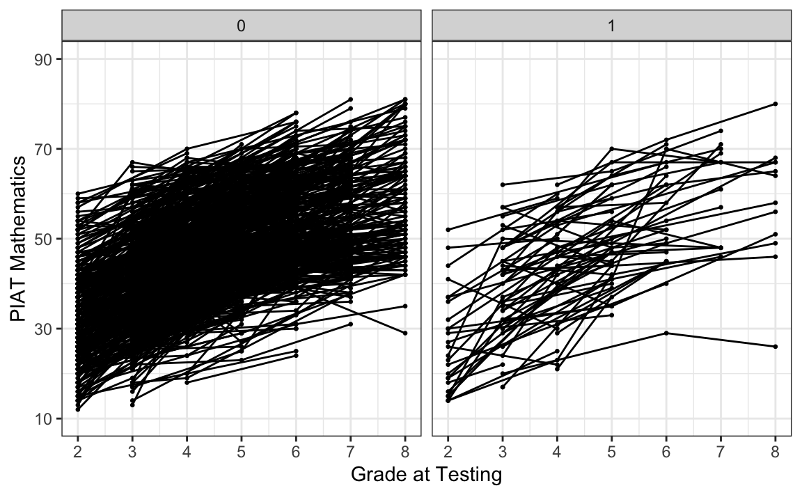
Per semplicità, carichiamo di nuovo i dati già trasformati in formato wide.
# set filepath for data file
filepath <- "https://raw.githubusercontent.com/LRI-2/Data/main/GrowthModeling/nlsy_math_wide_R.dat"
# read in the text data file using the url() function
dat <- read.table(
  file = url(filepath),
  na.strings = "."
) # indicates the missing data designator
# copy data with new name
nlsy_math_wide <- dat

# Give the variable names
names(nlsy_math_wide) <- c(
  "id", "female", "lb_wght", "anti_k1",
  "math2", "math3", "math4", "math5", "math6", "math7", "math8",
  "age2", "age3", "age4", "age5", "age6", "age7", "age8",
  "men2", "men3", "men4", "men5", "men6", "men7", "men8",
  "spring2", "spring3", "spring4", "spring5", "spring6", "spring7", "spring8",
  "anti2", "anti3", "anti4", "anti5", "anti6", "anti7", "anti8"
)

# view the first few observations (and columns) in the data set
head(nlsy_math_wide[, 1:11], 10)
#>      id female lb_wght anti_k1 math2 math3 math4 math5 math6 math7 math8
#> 1   201      1       0       0    NA    38    NA    55    NA    NA    NA
#> 2   303      1       0       1    26    NA    NA    33    NA    NA    NA
#> 3  2702      0       0       0    56    NA    58    NA    NA    NA    80
#> 4  4303      1       0       0    NA    41    58    NA    NA    NA    NA
#> 5  5002      0       0       4    NA    NA    46    NA    54    NA    66
#> 6  5005      1       0       0    35    NA    50    NA    60    NA    59
#> 7  5701      0       0       2    NA    62    61    NA    NA    NA    NA
#> 8  6102      0       0       0    NA    NA    55    67    NA    81    NA
#> 9  6801      1       0       0    NA    54    NA    62    NA    66    NA
#> 10 6802      0       0       0    NA    55    NA    66    NA    68    NA