33.1 Una applicazione concreta
L’approccio della finestra temporale è un metodo potenziale per analizzare dati con occasioni di misurazione individualmente variabili. In sostanza, l’approccio della finestra temporale mira ad approssimare la metrica del tempo individualmente variabile su una scala discreta. Ad esempio, ciò può essere ottenuto arrotondando il tempo/l’età al mezzo o al quarto d’anno più vicino.
Questo metodo è ovviamente ancora un’approssimazione del tempo. Si può ottenere maggiore precisione utilizzando finestre più piccole, ma se la matrice dei dati diventa troppo sparsa, la stima diventa difficile.
In questo esempio, le finestre temporali sono definite come semestri. Quindi, prendiamo i nostri dati in formato long, arrotondiamo l’età al semestre più vicino e convertiamo i dati in formato wide per l’utilizzo nel framework SEM.
Per questo esempio considereremo i dati di presrtazione matematica dal data set NLSY-CYA Long Data (si veda Grimm, Ram, and Estabrook 2016). Iniziamo a leggere i dati.
# set filepath for data file
filepath <- "https://raw.githubusercontent.com/LRI-2/Data/main/GrowthModeling/nlsy_math_long_R.dat"
# read in the text data file using the url() function
dat <- read.table(
file = url(filepath),
na.strings = "."
) # indicates the missing data designator
# copy data with new name
nlsy_math_long <- dat
# Add names the columns of the data set
names(nlsy_math_long) <- c(
"id", "female", "lb_wght",
"anti_k1", "math", "grade",
"occ", "age", "men",
"spring", "anti"
)
# subset to the variables of interest
nlsy_math_long <- nlsy_math_long[, c("id", "math", "grade", "age")]
# view the first few observations in the data set
head(nlsy_math_long, 10)
#> id math grade age
#> 1 201 38 3 111
#> 2 201 55 5 135
#> 3 303 26 2 121
#> 4 303 33 5 145
#> 5 2702 56 2 100
#> 6 2702 58 4 125
#> 7 2702 80 8 173
#> 8 4303 41 3 115
#> 9 4303 58 4 135
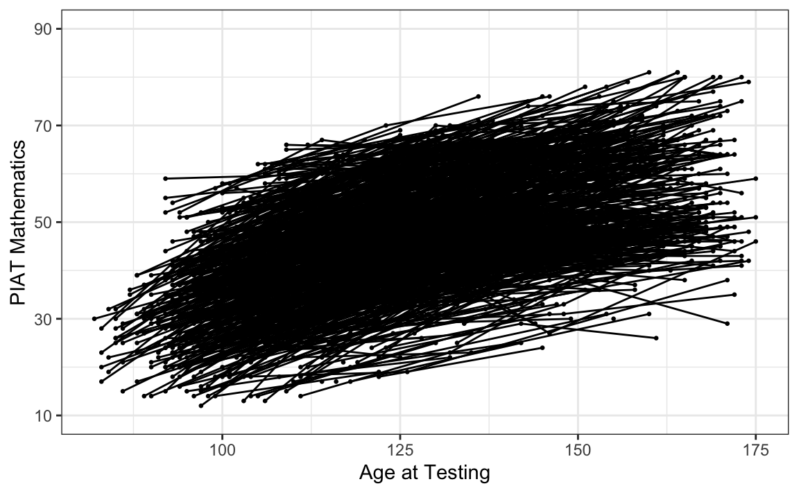
#> 10 5002 46 4 117# intraindividual change trajetories
ggplot(
data = nlsy_math_long, # data set
aes(x = age, y = math, group = id)
) + # setting variables
geom_point(size = .5) + # adding points to plot
geom_line() + # adding lines to plot
theme_bw() + # changing style/background
# setting the x-axis with breaks and labels
scale_x_continuous( # limits=c(2,8),
# breaks = c(2,3,4,5,6,7,8),
name = "Age at Testing"
) +
# setting the y-axis with limits breaks and labels
scale_y_continuous(
limits = c(10, 90),
breaks = c(10, 30, 50, 70, 90),
name = "PIAT Mathematics"
)
Implementiamo il metodo della finestra temporale e ricodifichiamo i dati in formato wide.
# creating new age variable scaled in years
nlsy_math_long$ageyr <- (nlsy_math_long$age / 12)
head(nlsy_math_long)
#>     id math grade age     ageyr
#> 1  201   38     3 111  9.250000
#> 2  201   55     5 135 11.250000
#> 3  303   26     2 121 10.083333
#> 4  303   33     5 145 12.083333
#> 5 2702   56     2 100  8.333333
#> 6 2702   58     4 125 10.416667
# rounding to nearest half-year
# multiplied by 10 to remove decimal for easy conversion to wide
nlsy_math_long$agewindow <- plyr::round_any(nlsy_math_long$ageyr * 10, 5)
head(nlsy_math_long)
#> id math grade age ageyr agewindow
#> 1 201 38 3 111 9.250000 90
#> 2 201 55 5 135 11.250000 110
#> 3 303 26 2 121 10.083333 100
#> 4 303 33 5 145 12.083333 120
#> 5 2702 56 2 100 8.333333 85
#> 6 2702 58 4 125 10.416667 105# reshaping long to wide (just variables of interest)
nlsy_math_wide <- reshape(
data = nlsy_math_long[, c("id", "math", "agewindow")],
timevar = c("agewindow"),
idvar = c("id"),
v.names = c("math"),
direction = "wide", sep = ""
)
# reordering columns for easy viewing
nlsy_math_wide <- nlsy_math_wide[, c(
"id", "math70", "math75", "math80", "math85", "math90", "math95", "math100", "math105", "math110", "math115", "math120", "math125", "math130", "math135", "math140", "math145"
)]
# looking at the data
head(nlsy_math_wide)
#> id math70 math75 math80 math85 math90 math95 math100 math105 math110
#> 1 201 NA NA NA NA 38 NA NA NA 55
#> 3 303 NA NA NA NA NA NA 26 NA NA
#> 5 2702 NA NA NA 56 NA NA NA 58 NA
#> 8 4303 NA NA NA NA NA 41 NA NA 58
#> 10 5002 NA NA NA NA NA NA 46 NA NA
#> 13 5005 NA NA 35 NA NA 50 NA NA NA
#> math115 math120 math125 math130 math135 math140 math145
#> 1 NA NA NA NA NA NA NA
#> 3 NA 33 NA NA NA NA NA
#> 5 NA NA NA NA NA NA 80
#> 8 NA NA NA NA NA NA NA
#> 10 NA 54 NA NA NA 66 NA
#> 13 60 NA NA NA 59 NA NASpecifichiamo il modello SEM.
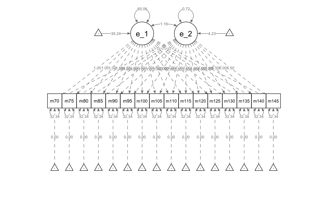
# writing out linear growth model in full SEM way
lg_math_age_lavaan_model <- "
  # latent variable definitions
      #intercept (note intercept is a reserved term)
      eta_1 =~ 1*math70 +
                1*math75 +
                1*math80 +
                1*math85 +
                1*math90 +
                1*math95 +
                1*math100 +
                1*math105 +
                1*math110 +
                1*math115 +
                1*math120 +
                1*math125 +
                1*math130 +
                1*math135 +
                1*math140 +
                1*math145

      #linear slope (note intercept is a reserved term)
      eta_2 =~ -1*math70 +
                -0.5*math75 +
                0*math80 +
                0.5*math85 +
                1*math90 +
                1.5*math95 +
                2*math100 +
                2.5*math105 +
                3*math110 +
                3.5*math115 +
                4*math120 +
                4.5*math125 +
                5*math130 +
                5.5*math135 +
                6*math140 +
                6.5*math145

  # factor variances
      eta_1 ~~ start(65)*eta_1
      eta_2 ~~ start(.75)*eta_2

  # covariances among factors
      eta_1 ~~ start(1.2)*eta_2

  # manifest variances (made equivalent by naming theta)
      math70 ~~ start(35)*theta*math70
      math75 ~~ theta*math75
      math80 ~~ theta*math80
      math85 ~~ theta*math85
      math90 ~~ theta*math90
      math95 ~~ theta*math95
      math100 ~~ theta*math100
      math105 ~~ theta*math105
      math110 ~~ theta*math110
      math115 ~~ theta*math115
      math120 ~~ theta*math120
      math125 ~~ theta*math125
      math130 ~~ theta*math130
      math135 ~~ theta*math135
      math140 ~~ theta*math140
      math145 ~~ theta*math145

  # manifest means (fixed at zero)
      math70 ~ 0*1
      math75 ~ 0*1
      math80 ~ 0*1
      math85 ~ 0*1
      math90 ~ 0*1
      math95 ~ 0*1
      math100 ~ 0*1
      math105 ~ 0*1
      math110 ~ 0*1
      math115 ~ 0*1
      math120 ~ 0*1
      math125 ~ 0*1
      math130 ~ 0*1
      math135 ~ 0*1
      math140 ~ 0*1
      math145 ~ 0*1

  # factor means (estimated freely)
      eta_1 ~ start(35)*1
      eta_2 ~ start(4)*1
" # end of model definition
Adattiamo il modello ai dati.
# estimating the model using sem() function
lg_math_age_lavaan_fit <- sem(lg_math_age_lavaan_model,
  data = nlsy_math_wide,
  meanstructure = TRUE,
  estimator = "ML",
  missing = "fiml"
)
Esaminiamo la soluzione.
summary(lg_math_age_lavaan_fit, fit.measures = TRUE)
#> lavaan 0.6.15 ended normally after 27 iterations
#>
#>   Estimator                                         ML
#>   Optimization method                           NLMINB
#>   Number of model parameters                        21
#>   Number of equality constraints                    15
#>
#>   Number of observations                           932
#>   Number of missing patterns                       139
#>
#> Model Test User Model:
#>
#>   Test statistic                               295.028
#>   Degrees of freedom                               146
#>   P-value (Chi-square)                           0.000
#>
#> Model Test Baseline Model:
#>
#>   Test statistic                              1053.342
#>   Degrees of freedom                               120
#>   P-value                                        0.000
#>
#> User Model versus Baseline Model:
#>
#>   Comparative Fit Index (CFI)                    0.840
#>   Tucker-Lewis Index (TLI)                       0.869
#>
#>   Robust Comparative Fit Index (CFI)             0.003
#>   Robust Tucker-Lewis Index (TLI)                0.181
#>
#> Loglikelihood and Information Criteria:
#>
#>   Loglikelihood user model (H0)              -7928.559
#>   Loglikelihood unrestricted model (H1)      -7781.045
#>
#>   Akaike (AIC)                               15869.117
#>   Bayesian (BIC)                             15898.141
#>   Sample-size adjusted Bayesian (SABIC)      15879.086
#>
#> Root Mean Square Error of Approximation:
#>
#>   RMSEA                                          0.033
#>   90 Percent confidence interval - lower         0.028
#>   90 Percent confidence interval - upper         0.039
#>   P-value H_0: RMSEA <= 0.050                    1.000
#>   P-value H_0: RMSEA >= 0.080                    0.000
#>
#>   Robust RMSEA                                   4.193
#>   90 Percent confidence interval - lower         0.000
#>   90 Percent confidence interval - upper         0.000
#>   P-value H_0: Robust RMSEA <= 0.050               NaN
#>   P-value H_0: Robust RMSEA >= 0.080               NaN
#>
#> Standardized Root Mean Square Residual:
#>
#>   SRMR                                           0.314
#>
#> Parameter Estimates:
#>
#>   Standard errors                             Standard
#>   Information                                 Observed
#>   Observed information based on                Hessian
#>
#> Latent Variables:
#>                    Estimate  Std.Err  z-value  P(>|z|)
#>   eta_1 =~
#>     math70            1.000
#>     math75            1.000
#>     math80            1.000
#>     math85            1.000
#>     math90            1.000
#>     math95            1.000
#>     math100           1.000
#>     math105           1.000
#>     math110           1.000
#>     math115           1.000
#>     math120           1.000
#>     math125           1.000
#>     math130           1.000
#>     math135           1.000
#>     math140           1.000
#>     math145           1.000
#>   eta_2 =~
#>     math70           -1.000
#>     math75           -0.500
#>     math80            0.000
#>     math85            0.500
#>     math90            1.000
#>     math95            1.500
#>     math100           2.000
#>     math105           2.500
#>     math110           3.000
#>     math115           3.500
#>     math120           4.000
#>     math125           4.500
#>     math130           5.000
#>     math135           5.500
#>     math140           6.000
#>     math145           6.500
#>
#> Covariances:
#>                    Estimate  Std.Err  z-value  P(>|z|)
#>   eta_1 ~~
#>     eta_2             1.157    1.010    1.146    0.252
#>
#> Intercepts:
#>                    Estimate  Std.Err  z-value  P(>|z|)
#>    .math70            0.000
#>    .math75            0.000
#>    .math80            0.000
#>    .math85            0.000
#>    .math90            0.000
#>    .math95            0.000
#>    .math100           0.000
#>    .math105           0.000
#>    .math110           0.000
#>    .math115           0.000
#>    .math120           0.000
#>    .math125           0.000
#>    .math130           0.000
#>    .math135           0.000
#>    .math140           0.000
#>    .math145           0.000
#>     eta_1            35.236    0.347  101.512    0.000
#>     eta_2             4.229    0.081   51.910    0.000
#>
#> Variances:
#>                    Estimate  Std.Err  z-value  P(>|z|)
#>     eta_1            65.063    5.503   11.824    0.000
#>     eta_2             0.725    0.277    2.616    0.009
#>    .math70  (thet)   32.337    1.695   19.083    0.000
#>    .math75  (thet)   32.337    1.695   19.083    0.000
#>    .math80  (thet)   32.337    1.695   19.083    0.000
#>    .math85  (thet)   32.337    1.695   19.083    0.000
#>    .math90  (thet)   32.337    1.695   19.083    0.000
#>    .math95  (thet)   32.337    1.695   19.083    0.000
#>    .math100 (thet)   32.337    1.695   19.083    0.000
#>    .math105 (thet)   32.337    1.695   19.083    0.000
#>    .math110 (thet)   32.337    1.695   19.083    0.000
#>    .math115 (thet)   32.337    1.695   19.083    0.000
#>    .math120 (thet)   32.337    1.695   19.083    0.000
#>    .math125 (thet)   32.337    1.695   19.083    0.000
#>    .math130 (thet)   32.337    1.695   19.083    0.000
#>    .math135 (thet)   32.337    1.695   19.083    0.000
#>    .math140 (thet)   32.337    1.695   19.083    0.000
#> .math145 (thet) 32.337 1.695 19.083 0.000parameterEstimates(lg_math_age_lavaan_fit)
#> lhs op rhs label est se z pvalue ci.lower ci.upper
#> 1 eta_1 =~ math70 1.000 0.000 NA NA 1.000 1.000
#> 2 eta_1 =~ math75 1.000 0.000 NA NA 1.000 1.000
#> 3 eta_1 =~ math80 1.000 0.000 NA NA 1.000 1.000
#> 4 eta_1 =~ math85 1.000 0.000 NA NA 1.000 1.000
#> 5 eta_1 =~ math90 1.000 0.000 NA NA 1.000 1.000
#> 6 eta_1 =~ math95 1.000 0.000 NA NA 1.000 1.000
#> 7 eta_1 =~ math100 1.000 0.000 NA NA 1.000 1.000
#> 8 eta_1 =~ math105 1.000 0.000 NA NA 1.000 1.000
#> 9 eta_1 =~ math110 1.000 0.000 NA NA 1.000 1.000
#> 10 eta_1 =~ math115 1.000 0.000 NA NA 1.000 1.000
#> 11 eta_1 =~ math120 1.000 0.000 NA NA 1.000 1.000
#> 12 eta_1 =~ math125 1.000 0.000 NA NA 1.000 1.000
#> 13 eta_1 =~ math130 1.000 0.000 NA NA 1.000 1.000
#> 14 eta_1 =~ math135 1.000 0.000 NA NA 1.000 1.000
#> 15 eta_1 =~ math140 1.000 0.000 NA NA 1.000 1.000
#> 16 eta_1 =~ math145 1.000 0.000 NA NA 1.000 1.000
#> 17 eta_2 =~ math70 -1.000 0.000 NA NA -1.000 -1.000
#> 18 eta_2 =~ math75 -0.500 0.000 NA NA -0.500 -0.500
#> 19 eta_2 =~ math80 0.000 0.000 NA NA 0.000 0.000
#> 20 eta_2 =~ math85 0.500 0.000 NA NA 0.500 0.500
#> 21 eta_2 =~ math90 1.000 0.000 NA NA 1.000 1.000
#> 22 eta_2 =~ math95 1.500 0.000 NA NA 1.500 1.500
#> 23 eta_2 =~ math100 2.000 0.000 NA NA 2.000 2.000
#> 24 eta_2 =~ math105 2.500 0.000 NA NA 2.500 2.500
#> 25 eta_2 =~ math110 3.000 0.000 NA NA 3.000 3.000
#> 26 eta_2 =~ math115 3.500 0.000 NA NA 3.500 3.500
#> 27 eta_2 =~ math120 4.000 0.000 NA NA 4.000 4.000
#> 28 eta_2 =~ math125 4.500 0.000 NA NA 4.500 4.500
#> 29 eta_2 =~ math130 5.000 0.000 NA NA 5.000 5.000
#> 30 eta_2 =~ math135 5.500 0.000 NA NA 5.500 5.500
#> 31 eta_2 =~ math140 6.000 0.000 NA NA 6.000 6.000
#> 32 eta_2 =~ math145 6.500 0.000 NA NA 6.500 6.500
#> 33 eta_1 ~~ eta_1 65.063 5.503 11.824 0.000 54.278 75.849
#> 34 eta_2 ~~ eta_2 0.725 0.277 2.616 0.009 0.182 1.268
#> 35 eta_1 ~~ eta_2 1.157 1.010 1.146 0.252 -0.822 3.136
#> 36 math70 ~~ math70 theta 32.337 1.695 19.083 0.000 29.016 35.658
#> 37 math75 ~~ math75 theta 32.337 1.695 19.083 0.000 29.016 35.658
#> 38 math80 ~~ math80 theta 32.337 1.695 19.083 0.000 29.016 35.658
#> 39 math85 ~~ math85 theta 32.337 1.695 19.083 0.000 29.016 35.658
#> 40 math90 ~~ math90 theta 32.337 1.695 19.083 0.000 29.016 35.658
#> 41 math95 ~~ math95 theta 32.337 1.695 19.083 0.000 29.016 35.658
#> 42 math100 ~~ math100 theta 32.337 1.695 19.083 0.000 29.016 35.658
#> 43 math105 ~~ math105 theta 32.337 1.695 19.083 0.000 29.016 35.658
#> 44 math110 ~~ math110 theta 32.337 1.695 19.083 0.000 29.016 35.658
#> 45 math115 ~~ math115 theta 32.337 1.695 19.083 0.000 29.016 35.658
#> 46 math120 ~~ math120 theta 32.337 1.695 19.083 0.000 29.016 35.658
#> 47 math125 ~~ math125 theta 32.337 1.695 19.083 0.000 29.016 35.658
#> 48 math130 ~~ math130 theta 32.337 1.695 19.083 0.000 29.016 35.658
#> 49 math135 ~~ math135 theta 32.337 1.695 19.083 0.000 29.016 35.658
#> 50 math140 ~~ math140 theta 32.337 1.695 19.083 0.000 29.016 35.658
#> 51 math145 ~~ math145 theta 32.337 1.695 19.083 0.000 29.016 35.658
#> 52 math70 ~1 0.000 0.000 NA NA 0.000 0.000
#> 53 math75 ~1 0.000 0.000 NA NA 0.000 0.000
#> 54 math80 ~1 0.000 0.000 NA NA 0.000 0.000
#> 55 math85 ~1 0.000 0.000 NA NA 0.000 0.000
#> 56 math90 ~1 0.000 0.000 NA NA 0.000 0.000
#> 57 math95 ~1 0.000 0.000 NA NA 0.000 0.000
#> 58 math100 ~1 0.000 0.000 NA NA 0.000 0.000
#> 59 math105 ~1 0.000 0.000 NA NA 0.000 0.000
#> 60 math110 ~1 0.000 0.000 NA NA 0.000 0.000
#> 61 math115 ~1 0.000 0.000 NA NA 0.000 0.000
#> 62 math120 ~1 0.000 0.000 NA NA 0.000 0.000
#> 63 math125 ~1 0.000 0.000 NA NA 0.000 0.000
#> 64 math130 ~1 0.000 0.000 NA NA 0.000 0.000
#> 65 math135 ~1 0.000 0.000 NA NA 0.000 0.000
#> 66 math140 ~1 0.000 0.000 NA NA 0.000 0.000
#> 67 math145 ~1 0.000 0.000 NA NA 0.000 0.000
#> 68 eta_1 ~1 35.236 0.347 101.512 0.000 34.556 35.917
#> 69 eta_2 ~1 4.229 0.081 51.910 0.000 4.069 4.389inspect(lg_math_age_lavaan_fit, what = "est")
#> $lambda
#> eta_1 eta_2
#> math70 1 -1.0
#> math75 1 -0.5
#> math80 1 0.0
#> math85 1 0.5
#> math90 1 1.0
#> math95 1 1.5
#> math100 1 2.0
#> math105 1 2.5
#> math110 1 3.0
#> math115 1 3.5
#> math120 1 4.0
#> math125 1 4.5
#> math130 1 5.0
#> math135 1 5.5
#> math140 1 6.0
#> math145 1 6.5
#>
#> $theta
#> math70 math75 math80 math85 math90 math95 mth100 mth105 mth110 mth115
#> math70 32.337
#> math75 0.000 32.337
#> math80 0.000 0.000 32.337
#> math85 0.000 0.000 0.000 32.337
#> math90 0.000 0.000 0.000 0.000 32.337
#> math95 0.000 0.000 0.000 0.000 0.000 32.337
#> math100 0.000 0.000 0.000 0.000 0.000 0.000 32.337
#> math105 0.000 0.000 0.000 0.000 0.000 0.000 0.000 32.337
#> math110 0.000 0.000 0.000 0.000 0.000 0.000 0.000 0.000 32.337
#> math115 0.000 0.000 0.000 0.000 0.000 0.000 0.000 0.000 0.000 32.337
#> math120 0.000 0.000 0.000 0.000 0.000 0.000 0.000 0.000 0.000 0.000
#> math125 0.000 0.000 0.000 0.000 0.000 0.000 0.000 0.000 0.000 0.000
#> math130 0.000 0.000 0.000 0.000 0.000 0.000 0.000 0.000 0.000 0.000
#> math135 0.000 0.000 0.000 0.000 0.000 0.000 0.000 0.000 0.000 0.000
#> math140 0.000 0.000 0.000 0.000 0.000 0.000 0.000 0.000 0.000 0.000
#> math145 0.000 0.000 0.000 0.000 0.000 0.000 0.000 0.000 0.000 0.000
#> mth120 mth125 mth130 mth135 mth140 mth145
#> math70
#> math75
#> math80
#> math85
#> math90
#> math95
#> math100
#> math105
#> math110
#> math115
#> math120 32.337
#> math125 0.000 32.337
#> math130 0.000 0.000 32.337
#> math135 0.000 0.000 0.000 32.337
#> math140 0.000 0.000 0.000 0.000 32.337
#> math145 0.000 0.000 0.000 0.000 0.000 32.337
#>
#> $psi
#> eta_1 eta_2
#> eta_1 65.063
#> eta_2 1.157 0.725
#>
#> $nu
#> intrcp
#> math70 0
#> math75 0
#> math80 0
#> math85 0
#> math90 0
#> math95 0
#> math100 0
#> math105 0
#> math110 0
#> math115 0
#> math120 0
#> math125 0
#> math130 0
#> math135 0
#> math140 0
#> math145 0
#>
#> $alpha
#> intrcp
#> eta_1 35.236
#> eta_2 4.229Creiamo un diagramma di percorso.