38.6 Parallel Process Model
Esaminiamo ora un modello che include sia i termini lineari che quadratici (quando richiesti) delle variabili x e y.
full_model <-
  "
  # intercept & slope growth terms for X
  iX =~ 1*x1 + 1*x2 + 1*x3 + 1*x4
  sX =~ 0*x1 + 1*x2 + 2*x3 + 3*x4

  # intercept, slope, & quadratic terms for Y
  iY =~ 1*y1 + 1*y2 + 1*y3 + 1*y4
  sY =~ 0*y1 + 1*y2 + 2*y3 + 3*y4
  qY =~ 0*y1 + 1*y2 + 4*y3 + 9*y4

  # regress growth terms on predictor
  qY + iY + sX + iX ~ predictor
  sY ~ a1*predictor

  # regress outcome on growth terms
  outcome ~ iX + sX + iY + b1*sY + qY

  # testing indirect effect
  # predictor --> sY --> outcome
  predictor_sY_outcome := a1*b1
"
Adattiamo il modello ai dati.
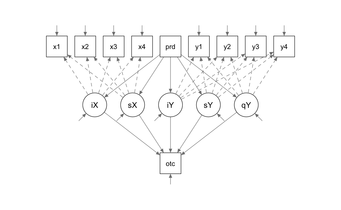
Esaminiamo il path diagram.
semPaths(
  full_fit,
  layout = "tree",
  intercepts = FALSE,
  posCol = c("black"),
  edge.label.cex = 0.00001,
  sizeMan = 7,
  what = "path",
  optimizeLatRes = TRUE,
  residuals = TRUE,
  style = "lisrel"
)
Valutiamo l’adattamento.
full_fit_stats <-
  fitmeasures(
    full_fit,
    selected_fit_stats
  )

round(full_fit_stats, 2)
#>        chisq.scaled           df.scaled       pvalue.scaled          cfi.scaled
#>               28.23               34.00                0.75                1.00
#>        rmsea.scaled rmsea.pvalue.scaled                srmr
#>                0.00                1.00                0.03
Si ottiene un ottimo adattamento del modello ai dati (il che non è sorprendente, in quanto i dati sono stati simulati in base a tale modello).