32.3 Modello di assenza di crescita
Sembra esserci una crescita sistematica nei punteggi di matematica nel tempo, come si può vedere nel nostro grafico sopra. Per iniziare l’analisi adatteremo un modello senza crescita. Questo modello senza crescita agirà come il nostro modello “nullo” a cui confrontare i modelli successivi.
Presentiamo il modello senza crescita perché è un punto di partenza comune e logico per qualsiasi studio del cambiamento poiché questo modello prevede che i punteggi non cambino con l’aumentare del tempo. Pertanto, il modello senza crescita è un modello che spesso vogliamo respingere. Il modello senza crescita ha una variabile latente, un’intercetta, che rappresenta il livello complessivo di prestazione nel tempo.
Impostiamo il modello senza crescita con la sintassi di lavaan.
# writing out no growth model in full SEM way
ng_math_lavaan_model <- "
  # latent variable definitions
      #intercept
      eta_1 =~ 1*math2
      eta_1 =~ 1*math3
      eta_1 =~ 1*math4
      eta_1 =~ 1*math5
      eta_1 =~ 1*math6
      eta_1 =~ 1*math7
      eta_1 =~ 1*math8

  # factor variances
      eta_1 ~~ eta_1

  # covariances among factors
      #none (only 1 factor)

  # factor means
      eta_1 ~ start(30)*1

  # manifest variances (made equivalent by naming theta)
      math2 ~~ theta*math2
      math3 ~~ theta*math3
      math4 ~~ theta*math4
      math5 ~~ theta*math5
      math6 ~~ theta*math6
      math7 ~~ theta*math7
      math8 ~~ theta*math8
  # manifest means (fixed at zero)
      math2 ~ 0*1
      math3 ~ 0*1
      math4 ~ 0*1
      math5 ~ 0*1
      math6 ~ 0*1
      math7 ~ 0*1
      math8 ~ 0*1
" # end of model definition
Adattiamo il modello ai dati.
ng_math_lavaan_fit <- sem(ng_math_lavaan_model,
  data = nlsy_math_wide,
  meanstructure = TRUE,
  estimator = "ML",
  missing = "fiml"
)
Esaminiamo la soluzione.
summary(ng_math_lavaan_fit, fit.measures = TRUE)
#> lavaan 0.6.15 ended normally after 18 iterations
#>
#> Estimator ML
#> Optimization method NLMINB
#> Number of model parameters 9
#> Number of equality constraints 6
#>
#> Used Total
#> Number of observations 932 933
#> Number of missing patterns 60
#>
#> Model Test User Model:
#>
#> Test statistic 1759.002
#> Degrees of freedom 32
#> P-value (Chi-square) 0.000
#>
#> Model Test Baseline Model:
#>
#> Test statistic 862.334
#> Degrees of freedom 21
#> P-value 0.000
#>
#> User Model versus Baseline Model:
#>
#> Comparative Fit Index (CFI) 0.000
#> Tucker-Lewis Index (TLI) -0.347
#>
#> Robust Comparative Fit Index (CFI) 0.000
#> Robust Tucker-Lewis Index (TLI) 0.093
#>
#> Loglikelihood and Information Criteria:
#>
#> Loglikelihood user model (H0) -8745.952
#> Loglikelihood unrestricted model (H1) -7866.451
#>
#> Akaike (AIC) 17497.903
#> Bayesian (BIC) 17512.415
#> Sample-size adjusted Bayesian (SABIC) 17502.888
#>
#> Root Mean Square Error of Approximation:
#>
#> RMSEA 0.241
#> 90 Percent confidence interval - lower 0.231
#> 90 Percent confidence interval - upper 0.250
#> P-value H_0: RMSEA <= 0.050 0.000
#> P-value H_0: RMSEA >= 0.080 1.000
#>
#> Robust RMSEA 0.467
#> 90 Percent confidence interval - lower 0.402
#> 90 Percent confidence interval - upper 0.534
#> P-value H_0: Robust RMSEA <= 0.050 0.000
#> P-value H_0: Robust RMSEA >= 0.080 1.000
#>
#> Standardized Root Mean Square Residual:
#>
#> SRMR 0.480
#>
#> Parameter Estimates:
#>
#> Standard errors Standard
#> Information Observed
#> Observed information based on Hessian
#>
#> Latent Variables:
#> Estimate Std.Err z-value P(>|z|)
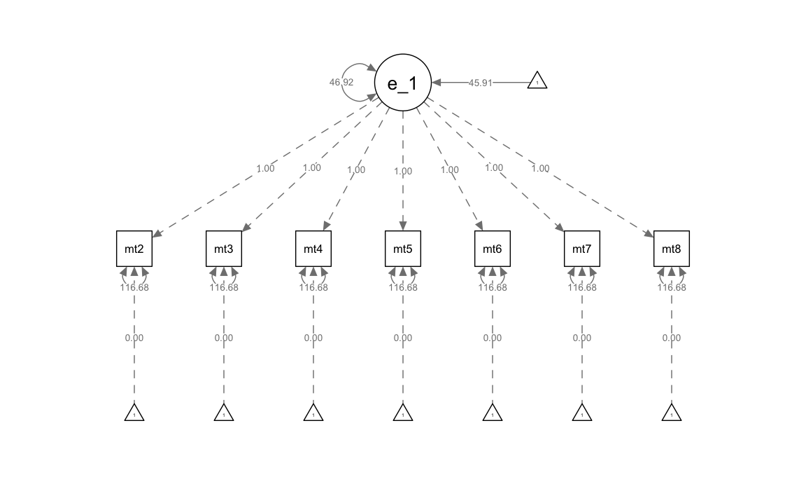
#> eta_1 =~
#> math2 1.000
#> math3 1.000
#> math4 1.000
#> math5 1.000
#> math6 1.000
#> math7 1.000
#> math8 1.000
#>
#> Intercepts:
#> Estimate Std.Err z-value P(>|z|)
#> eta_1 45.915 0.324 141.721 0.000
#> .math2 0.000
#> .math3 0.000
#> .math4 0.000
#> .math5 0.000
#> .math6 0.000
#> .math7 0.000
#> .math8 0.000
#>
#> Variances:
#> Estimate Std.Err z-value P(>|z|)
#> eta_1 46.917 4.832 9.709 0.000
#> .math2 (thet) 116.682 4.548 25.656 0.000
#> .math3 (thet) 116.682 4.548 25.656 0.000
#> .math4 (thet) 116.682 4.548 25.656 0.000
#> .math5 (thet) 116.682 4.548 25.656 0.000
#> .math6 (thet) 116.682 4.548 25.656 0.000
#> .math7 (thet) 116.682 4.548 25.656 0.000
#> .math8 (thet) 116.682 4.548 25.656 0.000Otteniamo il diagramma di percorso.
Calcoliamo le traiettorie predette.
# obtaining predicted factor scores for individuals
nlsy_math_predicted <- as.data.frame(cbind(nlsy_math_wide$id, lavPredict(ng_math_lavaan_fit)))

# naming columns
names(nlsy_math_predicted) <- c("id", "eta_1")

# looking at data
head(nlsy_math_predicted)
#>     id    eta_1
#> 1  201 46.17558
#> 2  303 38.59816
#> 3 2702 56.16725
#> 4 4303 47.51278
#> 5 5002 51.06429
#> 6 5005 49.05038
# calculating implied manifest scores
nlsy_math_predicted$math2 <- 1 * nlsy_math_predicted$eta_1
nlsy_math_predicted$math3 <- 1 * nlsy_math_predicted$eta_1
nlsy_math_predicted$math4 <- 1 * nlsy_math_predicted$eta_1
nlsy_math_predicted$math5 <- 1 * nlsy_math_predicted$eta_1
nlsy_math_predicted$math6 <- 1 * nlsy_math_predicted$eta_1
nlsy_math_predicted$math7 <- 1 * nlsy_math_predicted$eta_1
nlsy_math_predicted$math8 <- 1 * nlsy_math_predicted$eta_1
# reshaping wide to long
nlsy_math_predicted_long <- reshape(
data = nlsy_math_predicted,
timevar = c("grade"),
idvar = "id",
varying = c(
"math2", "math3", "math4",
"math5", "math6", "math7", "math8"
),
direction = "long", sep = ""
)
# sorting for easy viewing
# order by id and time
nlsy_math_predicted_long <- nlsy_math_predicted_long[order(nlsy_math_predicted_long$id, nlsy_math_predicted_long$grade), ]
# intraindividual change trajetories
ggplot(
data = nlsy_math_predicted_long, # data set
aes(x = grade, y = math, group = id)
) + # setting variables
# geom_point(size=.5) + #adding points to plot
geom_line() + # adding lines to plot
theme_bw() + # changing style/background
# setting the x-axis with breaks and labels
scale_x_continuous(
limits = c(2, 8),
breaks = c(2, 3, 4, 5, 6, 7, 8),
name = "Grade at Testing"
) +
# setting the y-axis with limits breaks and labels
scale_y_continuous(
limits = c(10, 90),
breaks = c(10, 30, 50, 70, 90),
name = "Predicted PIAT Mathematics"
)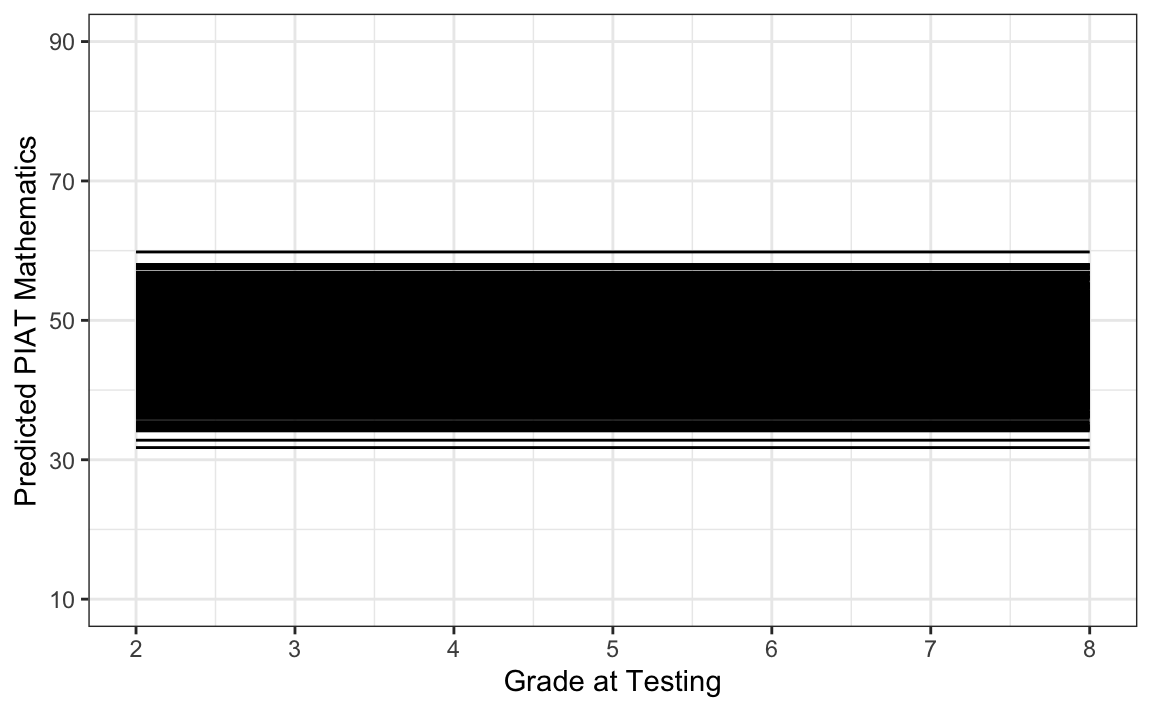
Vediamo dal grafico che il modello, come richiesto, produce una traiettoria di crescita piatta per ciascun individuo.