35.1 Invarianza tra gruppi
Definiamo il modello di crescita latente per i due gruppi.
# writing out linear growth model in full SEM way
mg_math_lavaan_model <- "
# latent variable definitions
#intercept (note intercept is a reserved term)
eta_1 =~ 1*math2
eta_1 =~ 1*math3
eta_1 =~ 1*math4
eta_1 =~ 1*math5
eta_1 =~ 1*math6
eta_1 =~ 1*math7
eta_1 =~ 1*math8
#linear slope
eta_2 =~ 0*math2
eta_2 =~ 1*math3
eta_2 =~ 2*math4
eta_2 =~ 3*math5
eta_2 =~ 4*math6
eta_2 =~ 5*math7
eta_2 =~ 6*math8
# factor variances
eta_1 ~~ eta_1
eta_2 ~~ eta_2
# covariances among factors
eta_1 ~~ eta_2
# factor means
eta_1 ~ start(35)*1
eta_2 ~ start(4)*1
# manifest variances (made equivalent by naming theta)
math2 ~~ theta*math2
math3 ~~ theta*math3
math4 ~~ theta*math4
math5 ~~ theta*math5
math6 ~~ theta*math6
math7 ~~ theta*math7
math8 ~~ theta*math8
# manifest means (fixed at zero)
math2 ~ 0*1
math3 ~ 0*1
math4 ~ 0*1
math5 ~ 0*1
math6 ~ 0*1
math7 ~ 0*1
math8 ~ 0*1
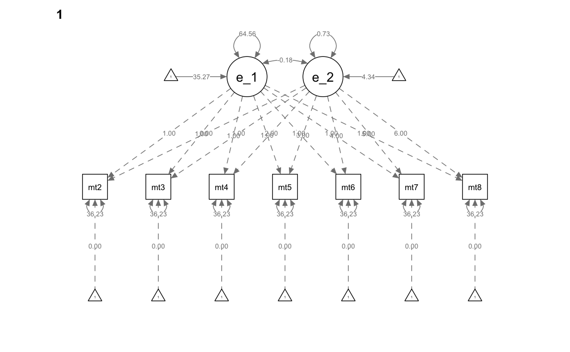
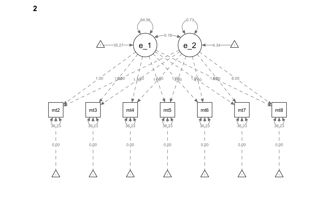
" # end of model definitionAdattiamo il modello ai dati specificando la separazione delle osservazioni in due gruppi e introducendo i vincoli di eguaglianza tra gruppi sulle saturazioni fattoriali, le medie, le varianze, le covarianze, e i residui. In questo modello, sostanzialmente, non c’è alcune differenza tra gruppi.
mg_math_lavaan_fitM1 <- sem(mg_math_lavaan_model,
  data = nlsy_math_wide,
  meanstructure = TRUE,
  estimator = "ML",
  missing = "fiml",
  group = "lb_wght", # to separate groups
  group.equal = c(
    "loadings", # for constraints
    "means",
    "lv.variances",
    "lv.covariances",
    "residuals"
  )
)
Esaminiamo il risultato
summary(mg_math_lavaan_fitM1, fit.measures = TRUE)
#> lavaan 0.6.15 ended normally after 24 iterations
#>
#>   Estimator                                         ML
#>   Optimization method                           NLMINB
#>   Number of model parameters                        24
#>   Number of equality constraints                    18
#>
#>   Number of observations per group:               Used       Total
#>     0                                              857         858
#>     1                                               75          75
#>   Number of missing patterns per group:
#>     0                                               60
#>     1                                               25
#>
#> Model Test User Model:
#>
#>   Test statistic                               249.111
#>   Degrees of freedom                                64
#>   P-value (Chi-square)                           0.000
#>   Test statistic for each group:
#>     0                                          191.954
#>     1                                           57.156
#>
#> Model Test Baseline Model:
#>
#>   Test statistic                               887.887
#>   Degrees of freedom                                42
#>   P-value                                        0.000
#>
#> User Model versus Baseline Model:
#>
#>   Comparative Fit Index (CFI)                    0.781
#>   Tucker-Lewis Index (TLI)                       0.856
#>
#>   Robust Comparative Fit Index (CFI)             1.000
#>   Robust Tucker-Lewis Index (TLI)                0.346
#>
#> Loglikelihood and Information Criteria:
#>
#>   Loglikelihood user model (H0)              -7968.693
#>   Loglikelihood unrestricted model (H1)      -7844.138
#>
#>   Akaike (AIC)                               15949.386
#>   Bayesian (BIC)                             15978.410
#>   Sample-size adjusted Bayesian (SABIC)      15959.354
#>
#> Root Mean Square Error of Approximation:
#>
#>   RMSEA                                          0.079
#>   90 Percent confidence interval - lower         0.069
#>   90 Percent confidence interval - upper         0.089
#>   P-value H_0: RMSEA <= 0.050                    0.000
#>   P-value H_0: RMSEA >= 0.080                    0.436
#>
#>   Robust RMSEA                                   0.000
#>   90 Percent confidence interval - lower         0.000
#>   90 Percent confidence interval - upper         0.000
#>   P-value H_0: Robust RMSEA <= 0.050             1.000
#>   P-value H_0: Robust RMSEA >= 0.080             0.000
#>
#> Standardized Root Mean Square Residual:
#>
#>   SRMR                                           0.128
#>
#> Parameter Estimates:
#>
#>   Standard errors                             Standard
#>   Information                                 Observed
#>   Observed information based on                Hessian
#>
#>
#> Group 1 [0]:
#>
#> Latent Variables:
#>                    Estimate  Std.Err  z-value  P(>|z|)
#>   eta_1 =~
#>     math2             1.000
#>     math3             1.000
#>     math4             1.000
#>     math5             1.000
#>     math6             1.000
#>     math7             1.000
#>     math8             1.000
#>   eta_2 =~
#>     math2             0.000
#>     math3             1.000
#>     math4             2.000
#>     math5             3.000
#>     math6             4.000
#>     math7             5.000
#>     math8             6.000
#>
#> Covariances:
#>                    Estimate  Std.Err  z-value  P(>|z|)
#>   eta_1 ~~
#>     eta_2   (.17.)   -0.181    1.150   -0.158    0.875
#>
#> Intercepts:
#>                    Estimate  Std.Err  z-value  P(>|z|)
#>     eta_1   (.18.)   35.267    0.355   99.229    0.000
#>     eta_2   (.19.)    4.339    0.088   49.136    0.000
#>    .math2             0.000
#>    .math3             0.000
#>    .math4             0.000
#>    .math5             0.000
#>    .math6             0.000
#>    .math7             0.000
#>    .math8             0.000
#>
#> Variances:
#>                    Estimate  Std.Err  z-value  P(>|z|)
#>     eta_1   (.15.)   64.562    5.659   11.408    0.000
#>     eta_2   (.16.)    0.733    0.327    2.238    0.025
#>    .math2   (thet)   36.230    1.867   19.410    0.000
#>    .math3   (thet)   36.230    1.867   19.410    0.000
#>    .math4   (thet)   36.230    1.867   19.410    0.000
#>    .math5   (thet)   36.230    1.867   19.410    0.000
#>    .math6   (thet)   36.230    1.867   19.410    0.000
#>    .math7   (thet)   36.230    1.867   19.410    0.000
#>    .math8   (thet)   36.230    1.867   19.410    0.000
#>
#>
#> Group 2 [1]:
#>
#> Latent Variables:
#>                    Estimate  Std.Err  z-value  P(>|z|)
#>   eta_1 =~
#>     math2             1.000
#>     math3             1.000
#>     math4             1.000
#>     math5             1.000
#>     math6             1.000
#>     math7             1.000
#>     math8             1.000
#>   eta_2 =~
#>     math2             0.000
#>     math3             1.000
#>     math4             2.000
#>     math5             3.000
#>     math6             4.000
#>     math7             5.000
#>     math8             6.000
#>
#> Covariances:
#>                    Estimate  Std.Err  z-value  P(>|z|)
#>   eta_1 ~~
#>     eta_2   (.17.)   -0.181    1.150   -0.158    0.875
#>
#> Intercepts:
#>                    Estimate  Std.Err  z-value  P(>|z|)
#>     eta_1   (.18.)   35.267    0.355   99.229    0.000
#>     eta_2   (.19.)    4.339    0.088   49.136    0.000
#>    .math2             0.000
#>    .math3             0.000
#>    .math4             0.000
#>    .math5             0.000
#>    .math6             0.000
#>    .math7             0.000
#>    .math8             0.000
#>
#> Variances:
#>                    Estimate  Std.Err  z-value  P(>|z|)
#>     eta_1   (.15.)   64.562    5.659   11.408    0.000
#>     eta_2   (.16.)    0.733    0.327    2.238    0.025
#>    .math2   (thet)   36.230    1.867   19.410    0.000
#>    .math3   (thet)   36.230    1.867   19.410    0.000
#>    .math4   (thet)   36.230    1.867   19.410    0.000
#>    .math5   (thet)   36.230    1.867   19.410    0.000
#>    .math6   (thet)   36.230    1.867   19.410    0.000
#>    .math7   (thet)   36.230    1.867   19.410    0.000
#>    .math8   (thet)   36.230    1.867   19.410    0.000
Creiamo il diagramma di percorso.