✏️ Esercizi#
In questo esercizio esamineremo i dati contenuti nel file MehrSongSpelke_exp_1.csv che sono stati messi a disposizione da Mehr, S. A., Song, L. A., & Spelke, E. S. nel loro articolo For 5-month-old infants. Questi dati sono descritti nell’esempio del laboratorio didattico presentato in queste pagine web. Nel presente esercizio ci concentreremo sui problemi della manipolazione e visualizzazione dei dati.
Iniziamo ad importare le librerie necessarie.
import numpy as np
import pandas as pd
import matplotlib.pyplot as plt
import seaborn as sns
from scipy import stats as stats

%config InlineBackend.figure_format = 'retina'
RANDOM_SEED = 42
rng = np.random.default_rng(RANDOM_SEED)

plt.style.use("https://raw.githubusercontent.com/NeuromatchAcademy/course-content/main/nma.mplstyle")
Importiamo i dati da un file csv.
tot_df = pd.read_csv("../chapter_0/laboratorio_didattico/MehrSongSpelke_exp_1.csv")
Esaminiamo a che classe (type) appartiene l’oggetto tot_df.
type(tot_df)
pandas.core.frame.DataFrame
L’output della funzione type ci dice che tot_df è un oggetto Pandas DataFrame.
Vogliamo poi sapere quante colonne e righe ci sono in tot_df. I nomi delle colonne sono restituiti dall’attributo .columns del DataFrame. Dato che il numero di colonne è molto grande, possiamo stamparle sullo schermo usando la sintassi seguente.
print(*tot_df.columns)
id study_code exp1 exp2 exp3 exp4 exp5 dob dot1 dot2 dot3 female dad train Baseline_Proportion_Gaze_to_Singer Familiarization_Gaze_to_Familiar Familiarization_Gaze_to_Unfamiliar Test_Proportion_Gaze_to_Singer Difference_in_Proportion_Looking Estimated_Total_Number_of_Song totskypesing stim othersing comply_no module skype_before ammat ammar ammatot ammapr ipad_num famtot_6 unfamtot_6 totprac totw totnw age length delay mtotsing mbabylike msingcomf mtotrecord m_othersong pright diarymissing comply_fup survey_completion smsingrate smtalkrate gzsingrate gztalkrate famtot unfamtot totsing1 babylike1 singcomf1 totrecord1 othersong1 dtword1 dtnoword1 totsing2 babylike2 singcomf2 totrecord2 othersong2 dtword2 dtnoword2 totsing3 babylike3 singcomf3 totrecord3 othersong3 dtword3 dtnoword3 totsing4 babylike4 singcomf4 totrecord4 othersong4 dtword4 dtnoword4 totsing5 babylike5 singcomf5 totrecord5 othersong5 dtword5 dtnoword5 totsing6 babylike6 singcomf6 totrecord6 othersong6 dtword6 dtnoword6 totsing7 babylike7 singcomf7 totrecord7 othersong7 dtword7 dtnoword7 totsing8 babylike8 singcomf8 totrecord8 othersong8 dtword8 dtnoword8 totsing9 babylike9 singcomf9 totrecord9 othersong9 dtword9 dtnoword9 totsing10 babylike10 singcomf10 totrecord10 othersong10 dtword10 dtnoword10 totsing11 babylike11 singcomf11 totrecord11 othersong11 dtword11 dtnoword11 totsing12 babylike12 singcomf12 totrecord12 othersong12 dtword12 dtnoword12 totsing13 babylike13 singcomf13 totrecord13 othersong13 dtword13 dtnoword13 totsing14 babylike14 singcomf14 totrecord14 othersong14 dtword14 dtnoword14 filter_$
L’attributo .shape ci restituisce l’informazione per cui l’oggetto tot_df è costituito da 96 righe e 153 colonne.
tot_df.shape
(96, 153)
È difficile lavorare con tutte queste colonne, per cui creeremo un DataFrame che contiene solo un sottoinsieme di colonne del DataFrame originale.
Per estrarre una singola colonna dal DataFrame usiamo la seguente sintassi. Ad esempio, estraiamo la colonna exp1.
tot_df["exp1"]
0     1
1     1
2     1
3     1
4     1
     ..
91    0
92    0
93    0
94    0
95    0
Name: exp1, Length: 96, dtype: int64
Si noti che una sintassi equivalente è la seguente.
tot_df.exp1
0     1
1     1
2     1
3     1
4     1
     ..
91    0
92    0
93    0
94    0
95    0
Name: exp1, Length: 96, dtype: int64
Con la funzione unique ottenamo la lista delle modalità di exp1.
tot_df["exp1"].unique()
array([1, 0])
Quindi, exp1 codifica l’appartenenza di ciascuna osservazione (valore 1) al primo esperimento; il valore 0 indica che la riga per la quale exp1 vale 0 non appartiene al primo esperimento.
Selezioniamo solo le colonne indicate. Si noti la sintassi con la doppia parentesi quadra. Le parentesi quadre interne specificano una lista.
temp = tot_df[["exp1", "female", "stim", "age", "Test_Proportion_Gaze_to_Singer"]]
temp.head()
| exp1 | female | stim | age | Test_Proportion_Gaze_to_Singer | |
|---|---|---|---|---|---|
| 0 | 1 | 0 | "C1" | 5.848049 | 0.602740 |
| 1 | 1 | 0 | "C1" | 5.979466 | 0.683027 |
| 2 | 1 | 0 | "C2" | 5.749486 | 0.724138 |
| 3 | 1 | 1 | "C3" | 5.913758 | 0.281654 |
| 4 | 1 | 1 | "C4" | 5.946612 | 0.498542 |
Selezioniamo solo le osservazioni dell’esperimento 1.
df = temp[temp["exp1"] == 1]
temp.head()
| exp1 | female | stim | age | Test_Proportion_Gaze_to_Singer | |
|---|---|---|---|---|---|
| 0 | 1 | 0 | "C1" | 5.848049 | 0.602740 |
| 1 | 1 | 0 | "C1" | 5.979466 | 0.683027 |
| 2 | 1 | 0 | "C2" | 5.749486 | 0.724138 |
| 3 | 1 | 1 | "C3" | 5.913758 | 0.281654 |
| 4 | 1 | 1 | "C4" | 5.946612 | 0.498542 |
Possiamo eliminare la colonna exp1 che ora è inutile.
df = df.drop(columns=["exp1"])
df.head()
| female | stim | age | Test_Proportion_Gaze_to_Singer | |
|---|---|---|---|---|
| 0 | 0 | "C1" | 5.848049 | 0.602740 |
| 1 | 0 | "C1" | 5.979466 | 0.683027 |
| 2 | 0 | "C2" | 5.749486 | 0.724138 |
| 3 | 1 | "C3" | 5.913758 | 0.281654 |
| 4 | 1 | "C4" | 5.946612 | 0.498542 |
df.tail()
| female | stim | age | Test_Proportion_Gaze_to_Singer | |
|---|---|---|---|---|
| 27 | 1 | "C4" | 5.355236 | 0.531100 |
| 28 | 0 | "C8" | 5.223819 | 0.541899 |
| 29 | 1 | "C5" | 6.045175 | 0.700389 |
| 30 | 1 | "C4" | 5.848049 | 0.762963 |
| 31 | 1 | "C6" | 5.420945 | 0.460274 |
Il DataFrame df è costituito da 32 righe e 4 colonne.
df.shape
(32, 4)
L’attributo dtypes ci restituisce il tipo di ciascuna colonna.
df.dtypes
female                              int64
stim                               object
age                               float64
Test_Proportion_Gaze_to_Singer    float64
dtype: object
La variabile
femaleè di tipo numerico e assume valori interi.La variabile
stimè una variabile categorica e le sue modalità sono rappresentate da stringhe.Le variabili
ageeTest_Proportion_Gaze_to_Singersono di tipo numerico e possono assumere valori decimali.
Selezionare le righe#
Le righe di un DataFrame possono essere selezionate usando il nome della riga o l’indice di riga.
È possibile utilizzare l’attributo .loc[] sul DataFrame per selezionare le righe in base all’etichetta dell’indice.
Selezioniamo la prima riga.
df.loc[0]
female                                   0
stim                                  "C1"
age                               5.848049
Test_Proportion_Gaze_to_Singer     0.60274
Name: 0, dtype: object
L’ultima riga.
df.loc[31]
female                                   1
stim                                  "C6"
age                               5.420945
Test_Proportion_Gaze_to_Singer    0.460274
Name: 31, dtype: object
Le prime 5 righe.
df.loc[0:4]
| female | stim | age | Test_Proportion_Gaze_to_Singer | |
|---|---|---|---|---|
| 0 | 0 | "C1" | 5.848049 | 0.602740 |
| 1 | 0 | "C1" | 5.979466 | 0.683027 |
| 2 | 0 | "C2" | 5.749486 | 0.724138 |
| 3 | 1 | "C3" | 5.913758 | 0.281654 |
| 4 | 1 | "C4" | 5.946612 | 0.498542 |
Le ultime 5 righe.
df.tail()
| female | stim | age | Test_Proportion_Gaze_to_Singer | |
|---|---|---|---|---|
| 27 | 1 | "C4" | 5.355236 | 0.531100 |
| 28 | 0 | "C8" | 5.223819 | 0.541899 |
| 29 | 1 | "C5" | 6.045175 | 0.700389 |
| 30 | 1 | "C4" | 5.848049 | 0.762963 |
| 31 | 1 | "C6" | 5.420945 | 0.460274 |
Le righe aventi l’indice 0, 3, 6, 9.
df.loc[[0, 3, 6, 9]]
| female | stim | age | Test_Proportion_Gaze_to_Singer | |
|---|---|---|---|---|
| 0 | 0 | "C1" | 5.848049 | 0.602740 |
| 3 | 1 | "C3" | 5.913758 | 0.281654 |
| 6 | 1 | "C6" | 5.486653 | 0.417755 |
| 9 | 1 | "C1" | 5.420945 | 0.586294 |
.iloc[] fa la stessa cosa di .loc[], ma viene utilizzato per selezionare le righe in base al numero dell’indice della riga. Nel nostro esempio attuale, .iloc[] e .loc[] si comporteranno esattamente allo stesso modo poiché le etichette degli indici sono i numeri delle righe. Tuttavia, bisogna tenere presente che le etichette degli indici non devono necessariamente essere i numeri delle righe.
Per esempio, ripetiamo l’ultima operazione.
df.iloc[[0, 3, 6, 9]]
| female | stim | age | Test_Proportion_Gaze_to_Singer | |
|---|---|---|---|---|
| 0 | 0 | "C1" | 5.848049 | 0.602740 |
| 3 | 1 | "C3" | 5.913758 | 0.281654 |
| 6 | 1 | "C6" | 5.486653 | 0.417755 |
| 9 | 1 | "C1" | 5.420945 | 0.586294 |
.iloc[] consente di selezionare simultaneamente righe e colonne. Per esempio, seleziamo tutte le righe delle colonne female e age. Poi stampiamo solo le prime 5 righe.
df.iloc[:, [0, 2]].head()
| female | age | |
|---|---|---|
| 0 | 0 | 5.848049 |
| 1 | 0 | 5.979466 |
| 2 | 0 | 5.749486 |
| 3 | 1 | 5.913758 |
| 4 | 1 | 5.946612 |
Statistiche descrittive#
Caloliamo la media della variabile Test_Proportion_Gaze_to_Singer.
df["Test_Proportion_Gaze_to_Singer"].mean()
0.59349125
Calcoliamo la deviazione standard quale statistica descrittiva.
df["Test_Proportion_Gaze_to_Singer"].std(ddof=0)
0.17587420037119572
Calcoliamo le statistiche elencate per le variabili age`` e Test_Proportion_Gaze_to_Singer`.
summary_stats = [np.min, np.median, np.mean, np.std, np.max]
result = df[["age", "Test_Proportion_Gaze_to_Singer"]].aggregate(summary_stats)
print(result)
             age  Test_Proportion_Gaze_to_Singer
min     5.059548                        0.262846
median  5.700205                        0.556953
mean    5.612936                        0.593491
std     0.312476                        0.178688
max     6.110883                        0.950920
/var/folders/cl/wwjrsxdd5tz7y9jr82nd5hrw0000gn/T/ipykernel_4353/3833652362.py:2: FutureWarning: The provided callable <function min at 0x1101f72e0> is currently using Series.min. In a future version of pandas, the provided callable will be used directly. To keep current behavior pass the string "min" instead.
  result = df[["age", "Test_Proportion_Gaze_to_Singer"]].aggregate(summary_stats)
/var/folders/cl/wwjrsxdd5tz7y9jr82nd5hrw0000gn/T/ipykernel_4353/3833652362.py:2: FutureWarning: The provided callable <function median at 0x110324d60> is currently using Series.median. In a future version of pandas, the provided callable will be used directly. To keep current behavior pass the string "median" instead.
  result = df[["age", "Test_Proportion_Gaze_to_Singer"]].aggregate(summary_stats)
/var/folders/cl/wwjrsxdd5tz7y9jr82nd5hrw0000gn/T/ipykernel_4353/3833652362.py:2: FutureWarning: The provided callable <function mean at 0x1101f7ba0> is currently using Series.mean. In a future version of pandas, the provided callable will be used directly. To keep current behavior pass the string "mean" instead.
  result = df[["age", "Test_Proportion_Gaze_to_Singer"]].aggregate(summary_stats)
/var/folders/cl/wwjrsxdd5tz7y9jr82nd5hrw0000gn/T/ipykernel_4353/3833652362.py:2: FutureWarning: The provided callable <function std at 0x1101f7ce0> is currently using Series.std. In a future version of pandas, the provided callable will be used directly. To keep current behavior pass the string "std" instead.
  result = df[["age", "Test_Proportion_Gaze_to_Singer"]].aggregate(summary_stats)
/var/folders/cl/wwjrsxdd5tz7y9jr82nd5hrw0000gn/T/ipykernel_4353/3833652362.py:2: FutureWarning: The provided callable <function max at 0x1101f71a0> is currently using Series.max. In a future version of pandas, the provided callable will be used directly. To keep current behavior pass the string "max" instead.
  result = df[["age", "Test_Proportion_Gaze_to_Singer"]].aggregate(summary_stats)
Ripetiamo i calcoli precedenti separatamente per maschi e femmine.
summary_stats = [np.min, np.median, np.mean, np.std, np.max]
result = df.groupby("female")[["age", "Test_Proportion_Gaze_to_Singer"]].aggregate(summary_stats)
print(result)
             age                                         \
             min    median      mean      std       max
female
0       5.059548  5.749486  5.563313  0.35660  6.110883
1       5.256673  5.552361  5.656722  0.27123  6.110883

       Test_Proportion_Gaze_to_Singer
                                  min    median      mean       std       max
female
0                            0.262846  0.542105  0.607096  0.214455  0.950920
1                            0.281654  0.571801  0.581487  0.145927  0.811189
/var/folders/cl/wwjrsxdd5tz7y9jr82nd5hrw0000gn/T/ipykernel_4353/4280065469.py:2: FutureWarning: The provided callable <function min at 0x1101f72e0> is currently using SeriesGroupBy.min. In a future version of pandas, the provided callable will be used directly. To keep current behavior pass the string "min" instead.
  result = df.groupby("female")[["age", "Test_Proportion_Gaze_to_Singer"]].aggregate(summary_stats)
/var/folders/cl/wwjrsxdd5tz7y9jr82nd5hrw0000gn/T/ipykernel_4353/4280065469.py:2: FutureWarning: The provided callable <function median at 0x110324d60> is currently using SeriesGroupBy.median. In a future version of pandas, the provided callable will be used directly. To keep current behavior pass the string "median" instead.
  result = df.groupby("female")[["age", "Test_Proportion_Gaze_to_Singer"]].aggregate(summary_stats)
/var/folders/cl/wwjrsxdd5tz7y9jr82nd5hrw0000gn/T/ipykernel_4353/4280065469.py:2: FutureWarning: The provided callable <function mean at 0x1101f7ba0> is currently using SeriesGroupBy.mean. In a future version of pandas, the provided callable will be used directly. To keep current behavior pass the string "mean" instead.
  result = df.groupby("female")[["age", "Test_Proportion_Gaze_to_Singer"]].aggregate(summary_stats)
/var/folders/cl/wwjrsxdd5tz7y9jr82nd5hrw0000gn/T/ipykernel_4353/4280065469.py:2: FutureWarning: The provided callable <function std at 0x1101f7ce0> is currently using SeriesGroupBy.std. In a future version of pandas, the provided callable will be used directly. To keep current behavior pass the string "std" instead.
  result = df.groupby("female")[["age", "Test_Proportion_Gaze_to_Singer"]].aggregate(summary_stats)
/var/folders/cl/wwjrsxdd5tz7y9jr82nd5hrw0000gn/T/ipykernel_4353/4280065469.py:2: FutureWarning: The provided callable <function max at 0x1101f71a0> is currently using SeriesGroupBy.max. In a future version of pandas, the provided callable will be used directly. To keep current behavior pass the string "max" instead.
  result = df.groupby("female")[["age", "Test_Proportion_Gaze_to_Singer"]].aggregate(summary_stats)
In maniera equivalente, possiamo usare la sintassi seguente. Si noti l’arrotondamento.
summary_stats = (
    df.loc[:, ["female", "age", "Test_Proportion_Gaze_to_Singer"]]
    .groupby(["female"])
    .aggregate([np.min, np.median, np.mean, np.std, np.max])
)
summary_stats.round(2)
/var/folders/cl/wwjrsxdd5tz7y9jr82nd5hrw0000gn/T/ipykernel_4353/3558284971.py:4: FutureWarning: The provided callable <function min at 0x1101f72e0> is currently using SeriesGroupBy.min. In a future version of pandas, the provided callable will be used directly. To keep current behavior pass the string "min" instead.
  .aggregate([np.min, np.median, np.mean, np.std, np.max])
/var/folders/cl/wwjrsxdd5tz7y9jr82nd5hrw0000gn/T/ipykernel_4353/3558284971.py:4: FutureWarning: The provided callable <function median at 0x110324d60> is currently using SeriesGroupBy.median. In a future version of pandas, the provided callable will be used directly. To keep current behavior pass the string "median" instead.
  .aggregate([np.min, np.median, np.mean, np.std, np.max])
/var/folders/cl/wwjrsxdd5tz7y9jr82nd5hrw0000gn/T/ipykernel_4353/3558284971.py:4: FutureWarning: The provided callable <function mean at 0x1101f7ba0> is currently using SeriesGroupBy.mean. In a future version of pandas, the provided callable will be used directly. To keep current behavior pass the string "mean" instead.
  .aggregate([np.min, np.median, np.mean, np.std, np.max])
/var/folders/cl/wwjrsxdd5tz7y9jr82nd5hrw0000gn/T/ipykernel_4353/3558284971.py:4: FutureWarning: The provided callable <function std at 0x1101f7ce0> is currently using SeriesGroupBy.std. In a future version of pandas, the provided callable will be used directly. To keep current behavior pass the string "std" instead.
  .aggregate([np.min, np.median, np.mean, np.std, np.max])
/var/folders/cl/wwjrsxdd5tz7y9jr82nd5hrw0000gn/T/ipykernel_4353/3558284971.py:4: FutureWarning: The provided callable <function max at 0x1101f71a0> is currently using SeriesGroupBy.max. In a future version of pandas, the provided callable will be used directly. To keep current behavior pass the string "max" instead.
  .aggregate([np.min, np.median, np.mean, np.std, np.max])
| age | Test_Proportion_Gaze_to_Singer | |||||||||
|---|---|---|---|---|---|---|---|---|---|---|
| min | median | mean | std | max | min | median | mean | std | max | |
| female | ||||||||||
| 0 | 5.06 | 5.75 | 5.56 | 0.36 | 6.11 | 0.26 | 0.54 | 0.61 | 0.21 | 0.95 |
| 1 | 5.26 | 5.55 | 5.66 | 0.27 | 6.11 | 0.28 | 0.57 | 0.58 | 0.15 | 0.81 |
Esaminimo il numero di maschi e femmine.
df.groupby(["female"]).size()
female
0    15
1    17
dtype: int64
Considerimo ora la variabile age.
df["age"]
0     5.848049
1     5.979466
2     5.749486
3     5.913758
4     5.946612
5     5.749486
6     5.486653
7     5.749486
8     6.110883
9     5.420945
10    6.110883
11    5.552361
12    5.749486
13    5.782341
14    5.815195
15    5.158111
16    5.256673
17    5.059548
18    5.190965
19    5.880904
20    5.256673
21    5.289528
22    5.552361
23    5.552361
24    5.650924
25    5.092402
26    5.815195
27    5.355236
28    5.223819
29    6.045175
30    5.848049
31    5.420945
Name: age, dtype: float64
Creiamo 5 classi che suddividendo i valori di questa variabile in 5 decili (il primo conterrà il 20% dei valori più bassi, ecc.).
df["age_deciles"] = pd.qcut(df["age"], 5, labels=False)
df["age_deciles"]
0     3
1     4
2     2
3     4
4     4
5     2
6     1
7     2
8     4
9     1
10    4
11    1
12    2
13    3
14    3
15    0
16    0
17    0
18    0
19    4
20    0
21    1
22    1
23    1
24    2
25    0
26    3
27    1
28    0
29    4
30    3
31    1
Name: age_deciles, dtype: int64
Calcoliamo la media dei valori Test_Proportion_Gaze_to_Singer in ciascuna delle 5 classi d’età.
prop_by_age = df.groupby('age_deciles')['Test_Proportion_Gaze_to_Singer'].mean()
prop_by_age
age_deciles
0    0.453139
1    0.584660
2    0.758172
3    0.722895
4    0.533876
Name: Test_Proportion_Gaze_to_Singer, dtype: float64
Rappresentiamo le medie di Test_Proportion_Gaze_to_Singer in funzoine delle 5 classi d’età.
prop_by_age.plot();
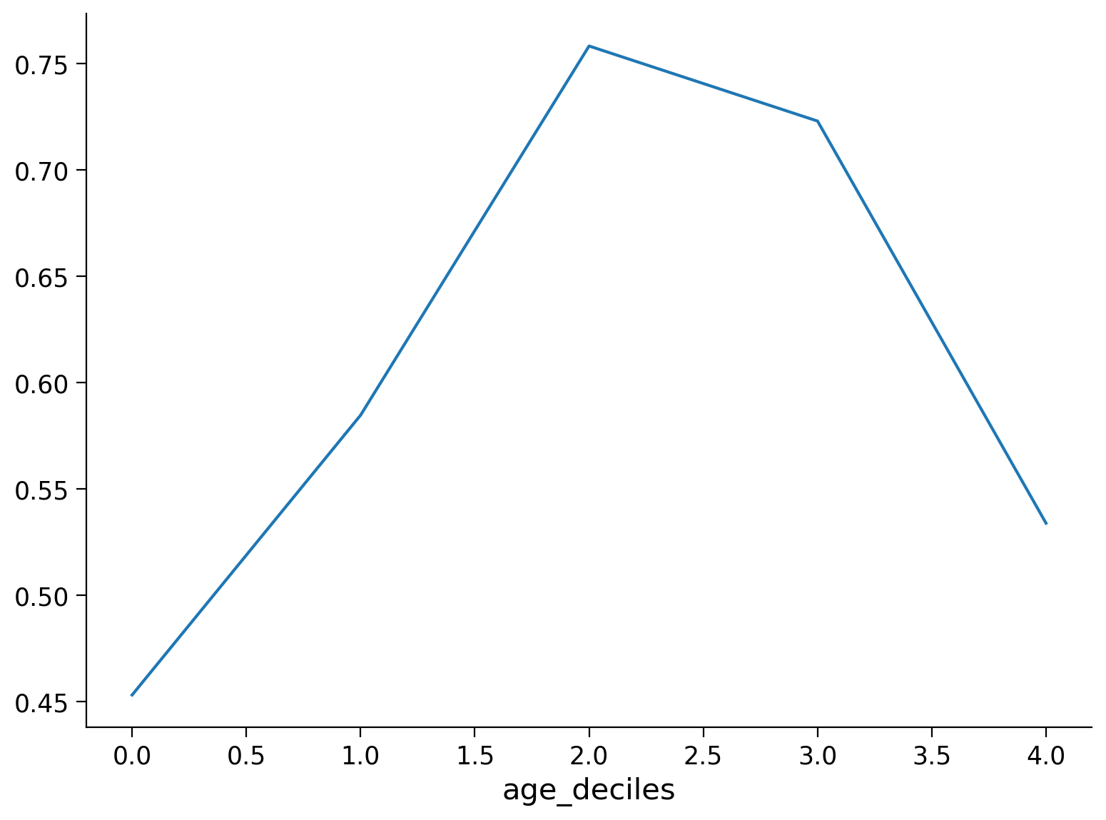
Non emerge alcuna tendenza degna di rilievo.
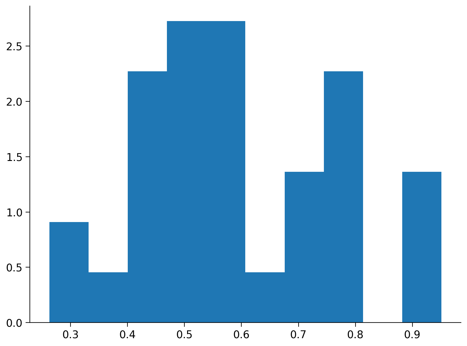
Creaimo un istogramma per la variabile Test_Proportion_Gaze_to_Singer.
plt.hist(df["Test_Proportion_Gaze_to_Singer"], density=True);
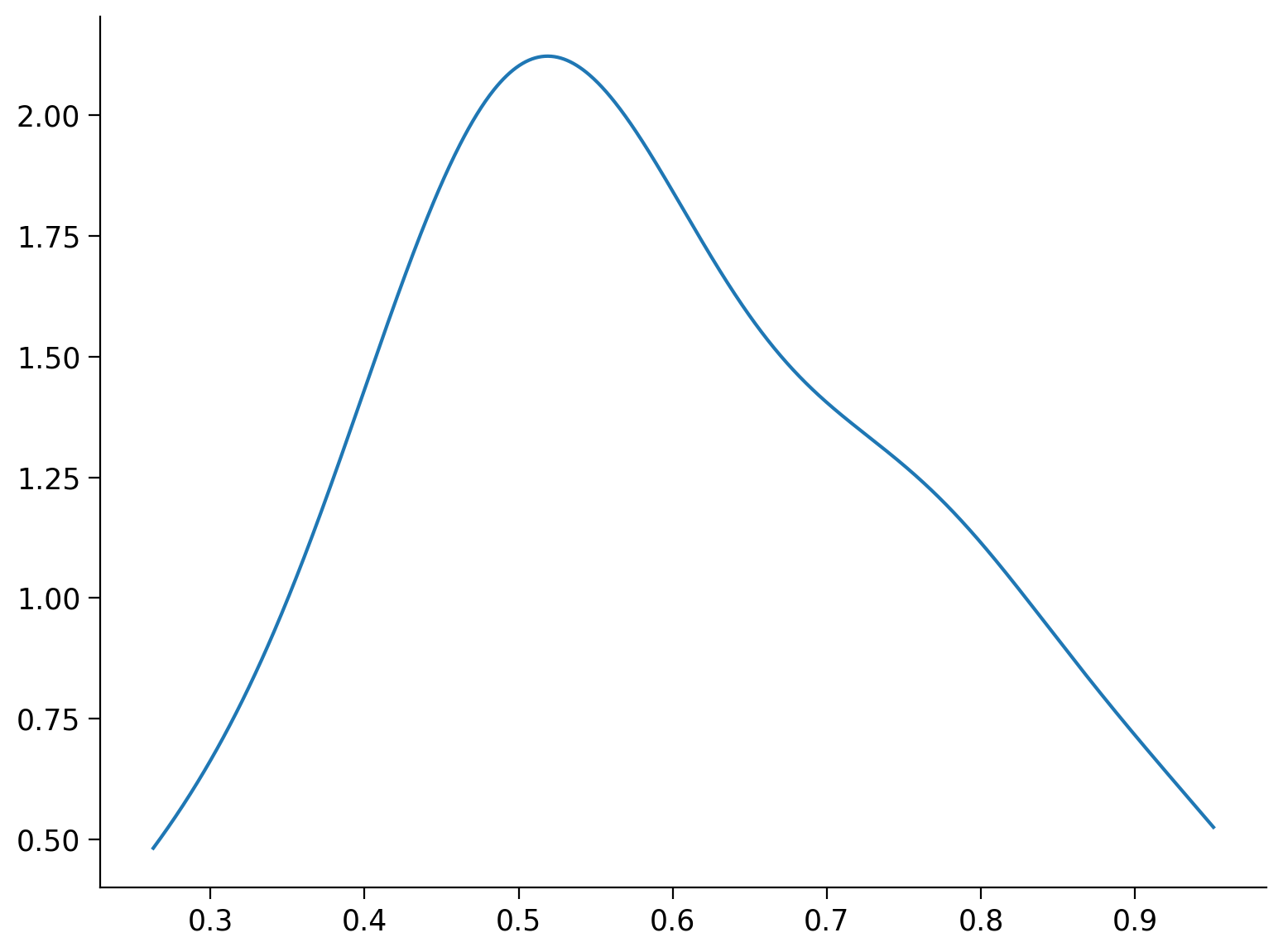
Rappresentiamo gli stessi dati con un KDE plot.
density = stats.gaussian_kde(df["Test_Proportion_Gaze_to_Singer"])
xs = np.linspace(min(df["Test_Proportion_Gaze_to_Singer"]), max(df["Test_Proportion_Gaze_to_Singer"]), 1000)
plt.plot(xs, density(xs));
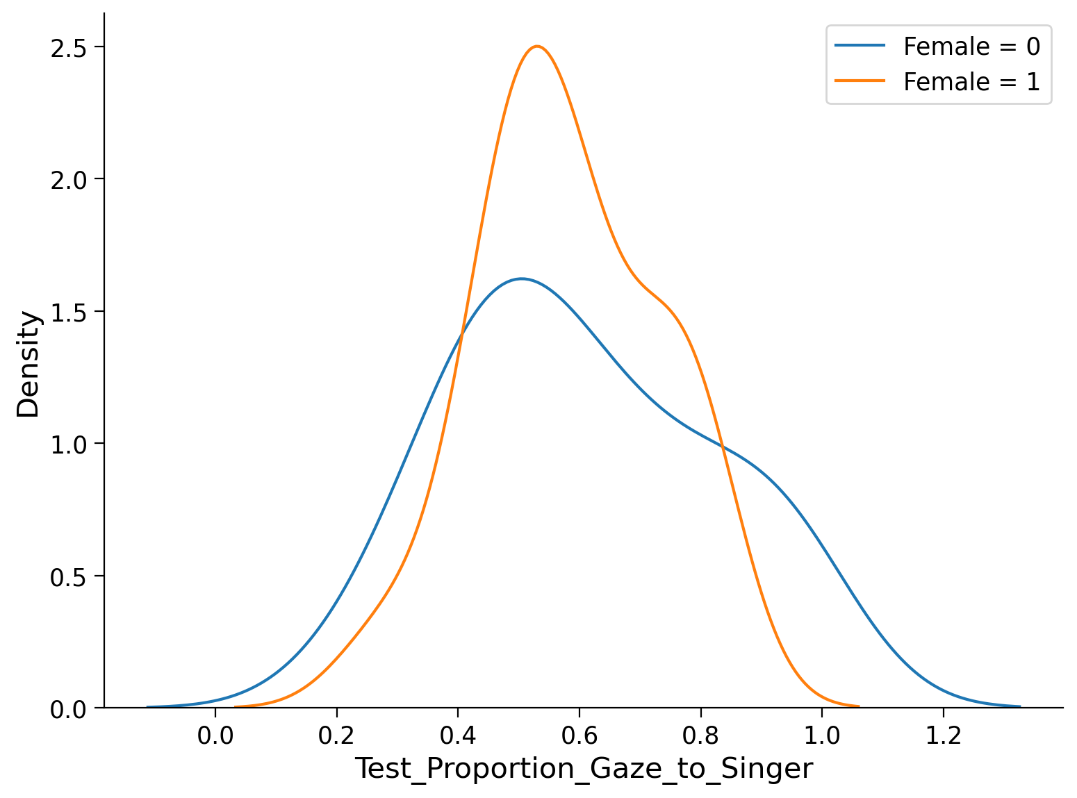
Usando seaborn è facile creare due KDE plot sovrapposti, uno per i maschi e uno per le femmine.
# KDE plot for female = 0 (or the first level)
sns.kdeplot(df[df["female"] == 0]["Test_Proportion_Gaze_to_Singer"], label='Female = 0')
# KDE plot for female = 1 (or the second level)
sns.kdeplot(df[df["female"] == 1]["Test_Proportion_Gaze_to_Singer"], label='Female = 1')
plt.legend();
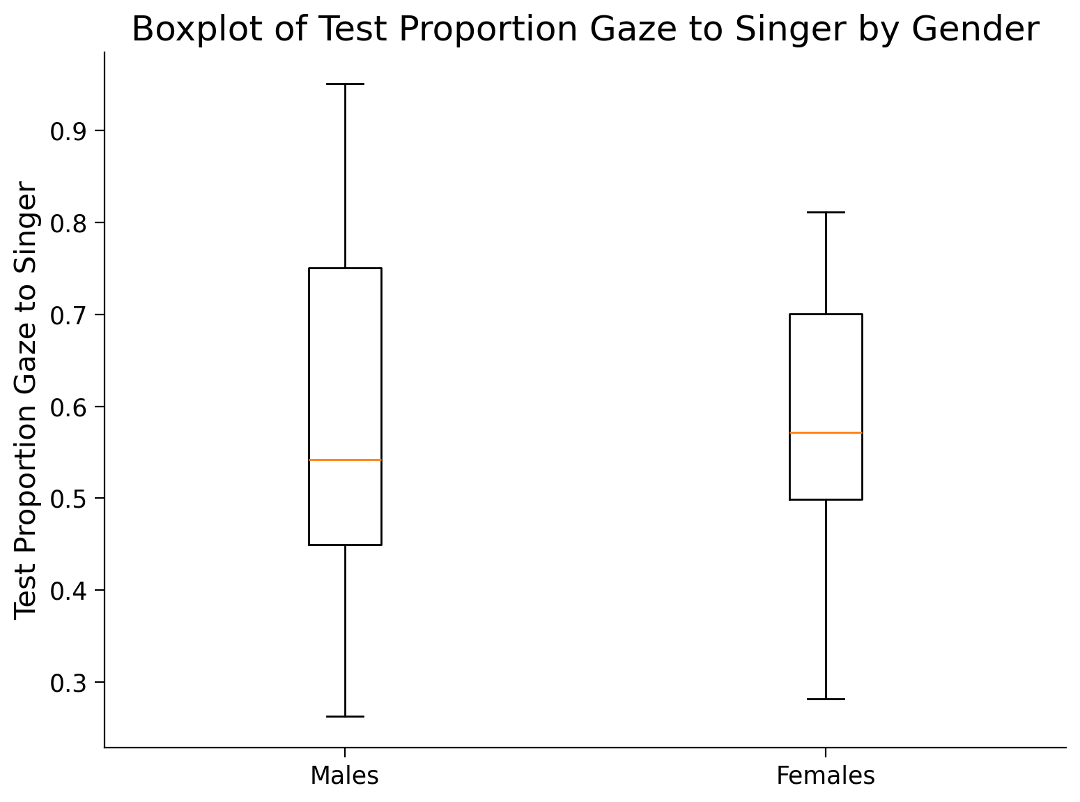
Creiamo due boxplot, uno per i maschi e uno per le femmine.
# Filter the data by the levels of the "female" variable
female_0 = df[df["female"] == 0]["Test_Proportion_Gaze_to_Singer"]
female_1 = df[df["female"] == 1]["Test_Proportion_Gaze_to_Singer"]

# Combine the filtered data
data = [female_0, female_1]

# Plot the boxplots
plt.boxplot(data, labels=['Males', 'Females'])

plt.title('Boxplot of Test Proportion Gaze to Singer by Gender')
plt.ylabel('Test Proportion Gaze to Singer');