Pandas (2)#
Il riepilogo dei dati in Pandas è un’attività fondamentale nell’analisi dei dati e consiste nel calcolare statistiche descrittive di un insieme di dati. In questo capitolo esamineremo come calcolare le statistiche descrittive di base usando Pandas (si veda il capitolo Indici di posizione e di scala).
Preparazione del Notebook#
import pandas as pd
import numpy as np
import matplotlib.pyplot as plt
from scipy import stats
import arviz as az
import seaborn as sns
%config InlineBackend.figure_format = 'retina'
RANDOM_SEED = 42
rng = np.random.default_rng(RANDOM_SEED)
az.style.use("arviz-darkgrid")
sns.set_theme(palette="colorblind")
Calcolo delle statistiche descrittive#
Agli oggetti Pandas possono essere applicati vari metodi matematici e statistici. La maggior parte di questi rientra nella categoria della riduzione di dati o delle statistiche descrittive. Rispetto ai metodi degli array NumPy, i metodi Pandas consentono la gestione dei dati mancanti. Alcuni dei metodi disponibili per gli oggetti Pandas sono elencati di seguito.
Method |
Description |
|---|---|
count |
Number of non-NA values |
describe |
Compute set of summary statistics |
min, max |
Compute minimum and maximum values |
argmin, argmax |
Compute index locations (integers) at which minimum or maximum value is obtained, respectively; not available on DataFrame objects |
idxmin, idxmax |
Compute index labels at which minimum or maximum value is obtained, respectively |
quantile |
Compute sample quantile ranging from 0 to 1 (default: 0.5) |
sum |
Sum of values |
mean |
Mean of values |
median |
Arithmetic median (50% quantile) of values |
mad |
Mean absolute deviation from mean value |
prod |
Product of all values |
var |
Sample variance of values |
std |
Sample standard deviation of values |
skew |
Sample skewness (third moment) of values |
kurt |
Sample kurtosis (fourth moment) of values |
cumsum |
Cumulative sum of values |
cummin, cummax |
Cumulative minimum or maximum of values, respectively |
cumprod |
Cumulative product of values |
diff |
Compute first arithmetic difference (useful for time series) |
pct_change |
Compute percent changes |
Tali metodi possono essere applicati a tutto il DataFrame, oppure soltanto ad una o più colonne.
Per fare un esempio, esamineremo nuovamente i dati penguins.csv. Come in precedenza, dopo avere caricato i dati, rimuoviamo i dati mancanti.
df = pd.read_csv("../data/penguins.csv")
df.dropna(inplace=True)
Usiamo il metodo describe() su tutto il DataFrame:
df.describe(include="all")
| species | island | bill_length_mm | bill_depth_mm | flipper_length_mm | body_mass_g | sex | year | |
|---|---|---|---|---|---|---|---|---|
| count | 333 | 333 | 333.000000 | 333.000000 | 333.000000 | 333.000000 | 333 | 333.000000 |
| unique | 3 | 3 | NaN | NaN | NaN | NaN | 2 | NaN |
| top | Adelie | Biscoe | NaN | NaN | NaN | NaN | male | NaN |
| freq | 146 | 163 | NaN | NaN | NaN | NaN | 168 | NaN |
| mean | NaN | NaN | 43.992793 | 17.164865 | 200.966967 | 4207.057057 | NaN | 2008.042042 |
| std | NaN | NaN | 5.468668 | 1.969235 | 14.015765 | 805.215802 | NaN | 0.812944 |
| min | NaN | NaN | 32.100000 | 13.100000 | 172.000000 | 2700.000000 | NaN | 2007.000000 |
| 25% | NaN | NaN | 39.500000 | 15.600000 | 190.000000 | 3550.000000 | NaN | 2007.000000 |
| 50% | NaN | NaN | 44.500000 | 17.300000 | 197.000000 | 4050.000000 | NaN | 2008.000000 |
| 75% | NaN | NaN | 48.600000 | 18.700000 | 213.000000 | 4775.000000 | NaN | 2009.000000 |
| max | NaN | NaN | 59.600000 | 21.500000 | 231.000000 | 6300.000000 | NaN | 2009.000000 |
Se desideriamo solo le informazioni relative alle variabili qualitative, usiamo l’argomento include='object'.
df.describe(include="object")
| species | island | sex | |
|---|---|---|---|
| count | 333 | 333 | 333 |
| unique | 3 | 3 | 2 |
| top | Adelie | Biscoe | male |
| freq | 146 | 163 | 168 |
I valori NaN indicano dati mancanti. Ad esempio, la colonna species contiene stringhe, quindi non esiste alcun valore per mean; allo stesso modo, bill_length_mm è una variabile numerica, quindi non vengono calcolate le statistiche riassuntive per le variabili categoriali (unique, top, freq).
Esaminimiamo le colonne singolarmente. Ad esempio, troviamo la media della colonna bill_depth_mm.
df["bill_depth_mm"].mean()
17.164864864864867
Per la deviazione standard usiamo il metodo std(). Si noti l’argomento opzionale ddof:
df["bill_length_mm"].std(ddof=1)
5.46866834264756
La cella seguente fornisce l’indice della riga nella quale la colonna bill_length_mm assume il suo valore massimo:
df["bill_length_mm"].idxmax()
185
La colonna species nel DataFrame df è una variabile a livello nominale. Elenchiamo le modalità di tale variabile.
df["species"].unique()
array(['Adelie', 'Gentoo', 'Chinstrap'], dtype=object)
Il metodo value_counts ritorna la distribuzione di frequenza assoluta:
df["species"].value_counts()
species
Adelie       146
Gentoo       119
Chinstrap     68
Name: count, dtype: int64
Per le frequenze relative si imposta l’argomento normalize=True:
print(df["species"].value_counts(normalize=True))
species
Adelie       0.438438
Gentoo       0.357357
Chinstrap    0.204204
Name: proportion, dtype: float64
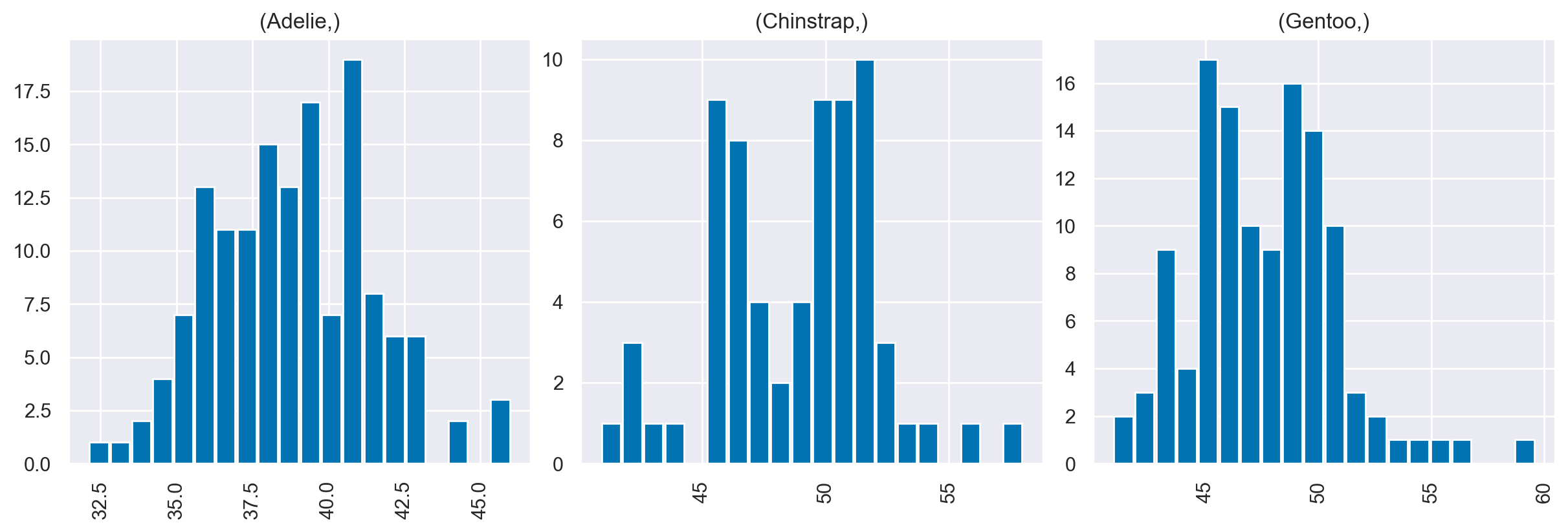
Consideriamo la lunghezza del becco dei pinguini suddivisa per ciascuna specie. Con l’istruzione seguente, possiamo generare gli istogrammi corrispondenti che rappresentano la distribuzione della lunghezza del becco in ciascun gruppo.
_ = df.hist(
    column="bill_length_mm",
    by=["species"],
    bins=20,
    figsize=(12, 4),
    layout=(1, 3),
    rwidth=0.9,
)
df
| species | island | bill_length_mm | bill_depth_mm | flipper_length_mm | body_mass_g | sex | year | |
|---|---|---|---|---|---|---|---|---|
| 0 | Adelie | Torgersen | 39.1 | 18.7 | 181.0 | 3750.0 | male | 2007 |
| 1 | Adelie | Torgersen | 39.5 | 17.4 | 186.0 | 3800.0 | female | 2007 |
| 2 | Adelie | Torgersen | 40.3 | 18.0 | 195.0 | 3250.0 | female | 2007 |
| 4 | Adelie | Torgersen | 36.7 | 19.3 | 193.0 | 3450.0 | female | 2007 |
| 5 | Adelie | Torgersen | 39.3 | 20.6 | 190.0 | 3650.0 | male | 2007 |
| ... | ... | ... | ... | ... | ... | ... | ... | ... |
| 339 | Chinstrap | Dream | 55.8 | 19.8 | 207.0 | 4000.0 | male | 2009 |
| 340 | Chinstrap | Dream | 43.5 | 18.1 | 202.0 | 3400.0 | female | 2009 |
| 341 | Chinstrap | Dream | 49.6 | 18.2 | 193.0 | 3775.0 | male | 2009 |
| 342 | Chinstrap | Dream | 50.8 | 19.0 | 210.0 | 4100.0 | male | 2009 |
| 343 | Chinstrap | Dream | 50.2 | 18.7 | 198.0 | 3775.0 | female | 2009 |
333 rows × 8 columns
Aggregazione dei dati#
Il riepilogo di più valori in un unico indice va sotto il nome di “aggregazione” dei dati. Il metodo aggregate() può essere applicato ai DataFrame e restituisce un nuovo DataFrame più breve contenente solo i valori aggregati. Il primo argomento di aggregate() specifica quale funzione o quali funzioni devono essere utilizzate per aggregare i dati. Molte comuni funzioni di aggregazione sono disponibili nel modulo statistics. Ad esempio:
median(): la mediana;mean(): la media;stdev(): la deviazione standard;
Se vogliamo applicare più funzioni di aggregazione, allora possiamo raccogliere prima le funzioni in una lista e poi passare la lista ad aggregate().
# List of summary statistics functions
summary_stats = [np.min, np.median, np.mean, np.std, np.max]

# Calculate summary statistics for numeric columns using aggregate
result = df[
    ["bill_length_mm", "bill_depth_mm", "flipper_length_mm", "body_mass_g"]
].aggregate(summary_stats)

print(result)
        bill_length_mm  bill_depth_mm  flipper_length_mm  body_mass_g
min          32.100000      13.100000         172.000000  2700.000000
median       44.500000      17.300000         197.000000  4050.000000
mean         43.992793      17.164865         200.966967  4207.057057
std           5.468668       1.969235          14.015765   805.215802
max          59.600000      21.500000         231.000000  6300.000000
/var/folders/cl/wwjrsxdd5tz7y9jr82nd5hrw0000gn/T/ipykernel_22725/3946289811.py:7: FutureWarning: The provided callable <function min at 0x111cf7420> is currently using Series.min. In a future version of pandas, the provided callable will be used directly. To keep current behavior pass the string "min" instead.
  ].aggregate(summary_stats)
/var/folders/cl/wwjrsxdd5tz7y9jr82nd5hrw0000gn/T/ipykernel_22725/3946289811.py:7: FutureWarning: The provided callable <function median at 0x111e20f40> is currently using Series.median. In a future version of pandas, the provided callable will be used directly. To keep current behavior pass the string "median" instead.
  ].aggregate(summary_stats)
/var/folders/cl/wwjrsxdd5tz7y9jr82nd5hrw0000gn/T/ipykernel_22725/3946289811.py:7: FutureWarning: The provided callable <function mean at 0x111cf7ce0> is currently using Series.mean. In a future version of pandas, the provided callable will be used directly. To keep current behavior pass the string "mean" instead.
  ].aggregate(summary_stats)
/var/folders/cl/wwjrsxdd5tz7y9jr82nd5hrw0000gn/T/ipykernel_22725/3946289811.py:7: FutureWarning: The provided callable <function std at 0x111cf7e20> is currently using Series.std. In a future version of pandas, the provided callable will be used directly. To keep current behavior pass the string "std" instead.
  ].aggregate(summary_stats)
/var/folders/cl/wwjrsxdd5tz7y9jr82nd5hrw0000gn/T/ipykernel_22725/3946289811.py:7: FutureWarning: The provided callable <function max at 0x111cf72e0> is currently using Series.max. In a future version of pandas, the provided callable will be used directly. To keep current behavior pass the string "max" instead.
  ].aggregate(summary_stats)
Si noti che Pandas ha applicato le funzioni di riepilogo a ogni colonna, ma, per alcune colonne, le statistiche riassuntive non si possono calcolare, ovvero tutte le colonne che contengono stringhe anziché numeri. Di conseguenza, vediamo che alcuni dei risultati per tali colonne sono contrassegnati con “NaN”. Questa è un’abbreviazione di “Not a Number”, talvolta utilizzata nell’analisi dei dati per rappresentare valori mancanti o non definiti.
Molto spesso vogliamo calcolare le statistiche descrittive separatamente per ciascun gruppo di osservazioni – per esempio, nel caso presente, potremmo volere distinguere le statistiche descrittive in base alla specie dei pinguini. Questo risultato si ottiene con il metodo .groupby().
Il nome “group by” deriva da un comando nel linguaggio del database SQL, ma forse è più semplice pensarlo nei termini coniati da Hadley Wickham: split, apply, combine. Un esempio canonico di questa operazione di split-apply-combine, in cui “apply” è un’aggregazione di sommatoria, è illustrato nella figura seguente:
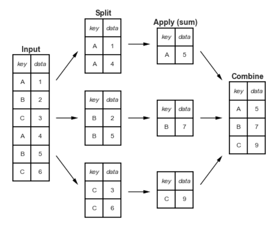
La figura rende chiaro ciò che si ottiene con groupby:
la fase “split” prevede la suddivisione e il raggruppamento di un DataFrame in base al valore della chiave specificata;
la fase “apply” implica il calcolo di alcune funzioni, solitamente un’aggregazione, una trasformazione o un filtro, all’interno dei singoli gruppi;
la fase “combine” unisce i risultati di queste operazioni in una matrice di output.
Per esempio, ragruppiamo le osservazioni body_mass_g in funzione delle modalità della variabile species.
grouped = df["body_mass_g"].groupby(df["species"])
Calcoliamo ora la media della variabile body_mass_g separatamente per ciascun gruppo di osservazioni.
grouped.mean()
species
Adelie       3706.164384
Chinstrap    3733.088235
Gentoo       5092.436975
Name: body_mass_g, dtype: float64
È possibile applicare criteri di classificazione multipli. Per fare un altro esempio, contiamo il numero di pinguini presenti sulle tre isole, distinguendoli per specie e genere.
df.groupby(["island", "species", "sex"]).size()
island     species    sex
Biscoe     Adelie     female    22
                      male      22
           Gentoo     female    58
                      male      61
Dream      Adelie     female    27
                      male      28
           Chinstrap  female    34
                      male      34
Torgersen  Adelie     female    24
                      male      23
dtype: int64
Con il metodo aggregate() possiamo applicare diverse funzioni di aggregazione alle osservazioni ragruppate. Ad esempio
summary_stats = [np.mean, np.std]
# Group by "species" and calculate summary statistics for numeric columns
result = df.groupby("species").agg(
    {col: summary_stats for col in df.columns if pd.api.types.is_numeric_dtype(df[col])}
)

print(result)
          bill_length_mm           bill_depth_mm           flipper_length_mm  \
                    mean       std          mean       std              mean
species
Adelie         38.823973  2.662597     18.347260  1.219338        190.102740
Chinstrap      48.833824  3.339256     18.420588  1.135395        195.823529
Gentoo         47.568067  3.106116     14.996639  0.985998        217.235294

                     body_mass_g                     year
                std         mean         std         mean       std
species
Adelie     6.521825  3706.164384  458.620135  2008.054795  0.811816
Chinstrap  7.131894  3733.088235  384.335081  2007.970588  0.863360
Gentoo     6.585431  5092.436975  501.476154  2008.067227  0.789025
/var/folders/cl/wwjrsxdd5tz7y9jr82nd5hrw0000gn/T/ipykernel_22725/259755461.py:3: FutureWarning: The provided callable <function mean at 0x111cf7ce0> is currently using SeriesGroupBy.mean. In a future version of pandas, the provided callable will be used directly. To keep current behavior pass the string "mean" instead.
  result = df.groupby("species").agg(
/var/folders/cl/wwjrsxdd5tz7y9jr82nd5hrw0000gn/T/ipykernel_22725/259755461.py:3: FutureWarning: The provided callable <function std at 0x111cf7e20> is currently using SeriesGroupBy.std. In a future version of pandas, the provided callable will be used directly. To keep current behavior pass the string "std" instead.
  result = df.groupby("species").agg(
/var/folders/cl/wwjrsxdd5tz7y9jr82nd5hrw0000gn/T/ipykernel_22725/259755461.py:3: FutureWarning: The provided callable <function mean at 0x111cf7ce0> is currently using SeriesGroupBy.mean. In a future version of pandas, the provided callable will be used directly. To keep current behavior pass the string "mean" instead.
  result = df.groupby("species").agg(
Nella cella seguente troviamo la media di body_mass_g e flipper_length_mm separatamente per ciascuna isola e ciascuna specie:
df.groupby(["island", "species"])[["body_mass_g", "flipper_length_mm"]].mean()
| body_mass_g | flipper_length_mm | ||
|---|---|---|---|
| island | species | ||
| Biscoe | Adelie | 3709.659091 | 188.795455 |
| Gentoo | 5092.436975 | 217.235294 | |
| Dream | Adelie | 3701.363636 | 189.927273 |
| Chinstrap | 3733.088235 | 195.823529 | |
| Torgersen | Adelie | 3708.510638 | 191.531915 |
Facciamo la stessa cosa per la deviazione standard.
df.groupby(["island", "species"])[["body_mass_g", "flipper_length_mm"]].std(ddof=1)
| body_mass_g | flipper_length_mm | ||
|---|---|---|---|
| island | species | ||
| Biscoe | Adelie | 487.733722 | 6.729247 |
| Gentoo | 501.476154 | 6.585431 | |
| Dream | Adelie | 448.774519 | 6.480325 |
| Chinstrap | 384.335081 | 7.131894 | |
| Torgersen | Adelie | 451.846351 | 6.220062 |
Prestiamo attenzione alla seguente sintassi:
summary_stats = (
    df.loc[:, ["island", "species", "body_mass_g", "flipper_length_mm"]]
    .groupby(["island", "species"])
    .aggregate(["mean", "std", "count"])
)
summary_stats
| body_mass_g | flipper_length_mm | ||||||
|---|---|---|---|---|---|---|---|
| mean | std | count | mean | std | count | ||
| island | species | ||||||
| Biscoe | Adelie | 3709.659091 | 487.733722 | 44 | 188.795455 | 6.729247 | 44 |
| Gentoo | 5092.436975 | 501.476154 | 119 | 217.235294 | 6.585431 | 119 | |
| Dream | Adelie | 3701.363636 | 448.774519 | 55 | 189.927273 | 6.480325 | 55 |
| Chinstrap | 3733.088235 | 384.335081 | 68 | 195.823529 | 7.131894 | 68 | |
| Torgersen | Adelie | 3708.510638 | 451.846351 | 47 | 191.531915 | 6.220062 | 47 |
Nell’istruzione precedente selezioniamo tutte le righe (:) di tre colonne di interesse: df.loc[:, ["island", "species", "body_mass_g", "flipper_length_mm"]]. L’istruzione .groupby(["island", "species"]) ragruppa le osservazioni (righe) secondo le modalità delle variabili island e species. Infine .aggregate(["mean", "std", "count"]) applica i metodi statistici specificati a ciascun gruppo di osservazioni. Con questa sintassi la sequenza delle operazioni da eseguire diventa molto intuitiva.
È possibile approfondire questo argomento consultanto il capitolo 10 del testo Python for Data Analysis di McKinney [McK22].
%load_ext watermark
%watermark -n -u -v -iv -w -m
Last updated: Mon Jan 29 2024

Python implementation: CPython
Python version       : 3.11.7
IPython version      : 8.19.0

Compiler    : Clang 16.0.6
OS          : Darwin
Release     : 23.3.0
Machine     : x86_64
Processor   : i386
CPU cores   : 8
Architecture: 64bit

seaborn   : 0.13.0
matplotlib: 3.8.2
pandas    : 2.1.4
numpy     : 1.26.2
scipy     : 1.11.4
arviz     : 0.17.0

Watermark: 2.4.3