here::here("code", "_common.R") |>
    source()

# Load packages
if (!requireNamespace("pacman")) install.packages("pacman")
pacman::p_load(DT, kableExtra, lme4, emmeans)80 Modelli di crescita latenti a gruppi multipli
Prerequisiti
Concetti e Competenze Chiave
Preparazione del Notebook
80.1 Introduzione
Nel capitolo precedente, abbiamo approfondito i modelli di crescita con covarianti invarianti nel tempo. In questo capitolo, esploreremo un approccio alternativo per studiare le differenze individuali nel cambiamento: l’analisi comparativa tra gruppi (McArdle, 1989; McArdle & Hamagami, 1996). Sebbene i modelli di crescita con covarianti invarianti nel tempo siano efficaci nell’analizzare le differenze nelle traiettorie medie di crescita, questi modelli presentano limitazioni nell’indagare altri aspetti dei cambiamenti intrapersonali e delle differenze interpersonali in tali processi.
Senza adeguati ampliamenti, i modelli basati esclusivamente su covarianti invarianti nel tempo non forniscono informazioni sulle variazioni nelle varianze e covarianze tra i fattori di crescita, né sulla variabilità residua e sulla dinamica dei cambiamenti intrapersonali. Nel presente capitolo, dimostreremo come l’approccio di confronto tra gruppi possa essere impiegato per esaminare le differenze in qualsiasi aspetto del modello di crescita. Questa flessibilità metodologica ci permette di acquisire una comprensione più profonda su come e perché gli individui mostrino percorsi di sviluppo diversificati.
Per i nostri esempi, utilizziamo i punteggi di rendimento in matematica dai dati NLSY-CYA [si veda {cite:t}grimm2016growth]. Importiamo i dati.
# set filepath for data file
filepath <- "https://raw.githubusercontent.com/LRI-2/Data/main/GrowthModeling/nlsy_math_long_R.dat"

# read in the text data file using the url() function
dat <- read.table(
  file = url(filepath),
  na.strings = "."
) # indicates the missing data designator

# copy data with new name
nlsy_math_long <- dat

# Add names the columns of the data set
names(nlsy_math_long) <- c(
  "id", "female", "lb_wght",
  "anti_k1", "math", "grade",
  "occ", "age", "men",
  "spring", "anti"
)

# reducing to variables of interest
nlsy_math_long <- nlsy_math_long[, c("id", "grade", "math", "lb_wght")]

# adding another dummy code variable for normal birth weight that coded the opposite of the low brithweight variable.
nlsy_math_long$nb_wght <- 1 - nlsy_math_long$lb_wght

# view the first few observations in the data set
head(nlsy_math_long, 10) |>
  print()
id grade math lb_wght nb_wght
1 201 3 38 0 1
2 201 5 55 0 1
3 303 2 26 0 1
4 303 5 33 0 1
5 2702 2 56 0 1
6 2702 4 58 0 1
7 2702 8 80 0 1
8 4303 3 41 0 1
9 4303 4 58 0 1
10 5002 4 46 0 1Esaminiamo le curve di crescita nei due gruppi.
# intraindividual change trajetories
ggplot(
  data = nlsy_math_long, # data set
  aes(x = grade, y = math, group = id)
) + # setting variables
  geom_point(size = .5) + # adding points to plot
  geom_line(alpha=0.3) + # adding lines to plot
  # setting the x-axis with breaks and labels
  scale_x_continuous(
    limits = c(2, 8),
    breaks = c(2, 3, 4, 5, 6, 7, 8),
    name = "Grade at Testing"
  ) +
  # setting the y-axis with limits breaks and labels
  scale_y_continuous(
    limits = c(10, 90),
    breaks = c(10, 30, 50, 70, 90),
    name = "PIAT Mathematics"
  ) +
  facet_wrap(~lb_wght)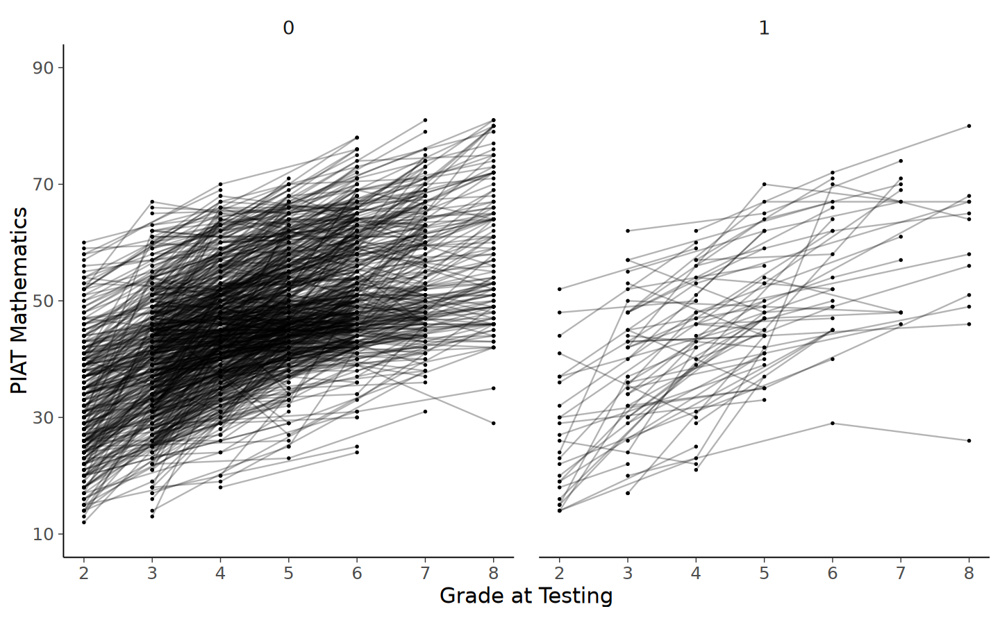
Per semplicità, carichiamo di nuovo i dati già trasformati in formato wide.
# set filepath for data file
filepath <- "https://raw.githubusercontent.com/LRI-2/Data/main/GrowthModeling/nlsy_math_wide_R.dat"
# read in the text data file using the url() function
dat <- read.table(
  file = url(filepath),
  na.strings = "."
) # indicates the missing data designator
# copy data with new name
nlsy_math_wide <- dat

# Give the variable names
names(nlsy_math_wide) <- c(
  "id", "female", "lb_wght", "anti_k1",
  "math2", "math3", "math4", "math5", "math6", "math7", "math8",
  "age2", "age3", "age4", "age5", "age6", "age7", "age8",
  "men2", "men3", "men4", "men5", "men6", "men7", "men8",
  "spring2", "spring3", "spring4", "spring5", "spring6", "spring7", "spring8",
  "anti2", "anti3", "anti4", "anti5", "anti6", "anti7", "anti8"
)

# view the first few observations (and columns) in the data set
head(nlsy_math_wide[, 1:11], 10)| id | female | lb_wght | anti_k1 | math2 | math3 | math4 | math5 | math6 | math7 | math8 | |
|---|---|---|---|---|---|---|---|---|---|---|---|
| <int> | <int> | <int> | <int> | <int> | <int> | <int> | <int> | <int> | <int> | <int> | |
| 1 | 201 | 1 | 0 | 0 | NA | 38 | NA | 55 | NA | NA | NA |
| 2 | 303 | 1 | 0 | 1 | 26 | NA | NA | 33 | NA | NA | NA |
| 3 | 2702 | 0 | 0 | 0 | 56 | NA | 58 | NA | NA | NA | 80 |
| 4 | 4303 | 1 | 0 | 0 | NA | 41 | 58 | NA | NA | NA | NA |
| 5 | 5002 | 0 | 0 | 4 | NA | NA | 46 | NA | 54 | NA | 66 |
| 6 | 5005 | 1 | 0 | 0 | 35 | NA | 50 | NA | 60 | NA | 59 |
| 7 | 5701 | 0 | 0 | 2 | NA | 62 | 61 | NA | NA | NA | NA |
| 8 | 6102 | 0 | 0 | 0 | NA | NA | 55 | 67 | NA | 81 | NA |
| 9 | 6801 | 1 | 0 | 0 | NA | 54 | NA | 62 | NA | 66 | NA |
| 10 | 6802 | 0 | 0 | 0 | NA | 55 | NA | 66 | NA | 68 | NA |
80.2 Invarianza tra gruppi
Definiamo il modello di crescita latente per i due gruppi.
# writing out linear growth model in full SEM way
mg_math_lavaan_model <- "
  # latent variable definitions
      #intercept (note intercept is a reserved term)
      eta_1 =~ 1*math2
      eta_1 =~ 1*math3
      eta_1 =~ 1*math4
      eta_1 =~ 1*math5
      eta_1 =~ 1*math6
      eta_1 =~ 1*math7
      eta_1 =~ 1*math8

      #linear slope
      eta_2 =~ 0*math2
      eta_2 =~ 1*math3
      eta_2 =~ 2*math4
      eta_2 =~ 3*math5
      eta_2 =~ 4*math6
      eta_2 =~ 5*math7
      eta_2 =~ 6*math8

  # factor variances
      eta_1 ~~ eta_1
      eta_2 ~~ eta_2

  # covariances among factors
      eta_1 ~~ eta_2

  # factor means
      eta_1 ~ start(35)*1
      eta_2 ~ start(4)*1

  # manifest variances (made equivalent by naming theta)
      math2 ~~ theta*math2
      math3 ~~ theta*math3
      math4 ~~ theta*math4
      math5 ~~ theta*math5
      math6 ~~ theta*math6
      math7 ~~ theta*math7
      math8 ~~ theta*math8
  # manifest means (fixed at zero)
      math2 ~ 0*1
      math3 ~ 0*1
      math4 ~ 0*1
      math5 ~ 0*1
      math6 ~ 0*1
      math7 ~ 0*1
      math8 ~ 0*1
" # end of model definition
Adattiamo il modello ai dati specificando la separazione delle osservazioni in due gruppi e introducendo i vincoli di eguaglianza tra gruppi sulle saturazioni fattoriali, le medie, le varianze, le covarianze, e i residui. In questo modello, sostanzialmente, non c’è alcune differenza tra gruppi.
mg_math_lavaan_fitM1 <- sem(mg_math_lavaan_model,
  data = nlsy_math_wide,
  meanstructure = TRUE,
  estimator = "ML",
  missing = "fiml",
  group = "lb_wght", # to separate groups
  group.equal = c(
    "loadings", # for constraints
    "means",
    "lv.variances",
    "lv.covariances",
    "residuals"
  )
)
Esaminiamo i risultati.
summary(mg_math_lavaan_fitM1, fit.measures = TRUE) |>
    print()
lavaan 0.6-19 ended normally after 24 iterations
Estimator ML
Optimization method NLMINB
Number of model parameters 24
Number of equality constraints 18
Number of observations per group: Used Total
0 857 858
1 75 75
Number of missing patterns per group:
0 60
1 25
Model Test User Model:
Test statistic 249.111
Degrees of freedom 64
P-value (Chi-square) 0.000
Test statistic for each group:
0 191.954
1 57.156
Model Test Baseline Model:
Test statistic 887.887
Degrees of freedom 42
P-value 0.000
User Model versus Baseline Model:
Comparative Fit Index (CFI) 0.781
Tucker-Lewis Index (TLI) 0.856
Robust Comparative Fit Index (CFI) 1.000
Robust Tucker-Lewis Index (TLI) 0.346
Loglikelihood and Information Criteria:
Loglikelihood user model (H0) -7968.693
Loglikelihood unrestricted model (H1) -7844.138
Akaike (AIC) 15949.386
Bayesian (BIC) 15978.410
Sample-size adjusted Bayesian (SABIC) 15959.354
Root Mean Square Error of Approximation:
RMSEA 0.079
90 Percent confidence interval - lower 0.069
90 Percent confidence interval - upper 0.089
P-value H_0: RMSEA <= 0.050 0.000
P-value H_0: RMSEA >= 0.080 0.436
Robust RMSEA 0.000
90 Percent confidence interval - lower 0.000
90 Percent confidence interval - upper 0.000
P-value H_0: Robust RMSEA <= 0.050 1.000
P-value H_0: Robust RMSEA >= 0.080 0.000
Standardized Root Mean Square Residual:
SRMR 0.128
Parameter Estimates:
Standard errors Standard
Information Observed
Observed information based on Hessian
Group 1 [0]:
Latent Variables:
Estimate Std.Err z-value P(>|z|)
eta_1 =~
math2 1.000
math3 1.000
math4 1.000
math5 1.000
math6 1.000
math7 1.000
math8 1.000
eta_2 =~
math2 0.000
math3 1.000
math4 2.000
math5 3.000
math6 4.000
math7 5.000
math8 6.000
Covariances:
Estimate Std.Err z-value P(>|z|)
eta_1 ~~
eta_2 (.17.) -0.181 1.150 -0.158 0.875
Intercepts:
Estimate Std.Err z-value P(>|z|)
eta_1 (.18.) 35.267 0.355 99.229 0.000
eta_2 (.19.) 4.339 0.088 49.136 0.000
.math2 0.000
.math3 0.000
.math4 0.000
.math5 0.000
.math6 0.000
.math7 0.000
.math8 0.000
Variances:
Estimate Std.Err z-value P(>|z|)
eta_1 (.15.) 64.562 5.659 11.408 0.000
eta_2 (.16.) 0.733 0.327 2.238 0.025
.math2 (thet) 36.230 1.867 19.410 0.000
.math3 (thet) 36.230 1.867 19.410 0.000
.math4 (thet) 36.230 1.867 19.410 0.000
.math5 (thet) 36.230 1.867 19.410 0.000
.math6 (thet) 36.230 1.867 19.410 0.000
.math7 (thet) 36.230 1.867 19.410 0.000
.math8 (thet) 36.230 1.867 19.410 0.000
Group 2 [1]:
Latent Variables:
Estimate Std.Err z-value P(>|z|)
eta_1 =~
math2 1.000
math3 1.000
math4 1.000
math5 1.000
math6 1.000
math7 1.000
math8 1.000
eta_2 =~
math2 0.000
math3 1.000
math4 2.000
math5 3.000
math6 4.000
math7 5.000
math8 6.000
Covariances:
Estimate Std.Err z-value P(>|z|)
eta_1 ~~
eta_2 (.17.) -0.181 1.150 -0.158 0.875
Intercepts:
Estimate Std.Err z-value P(>|z|)
eta_1 (.18.) 35.267 0.355 99.229 0.000
eta_2 (.19.) 4.339 0.088 49.136 0.000
.math2 0.000
.math3 0.000
.math4 0.000
.math5 0.000
.math6 0.000
.math7 0.000
.math8 0.000
Variances:
Estimate Std.Err z-value P(>|z|)
eta_1 (.15.) 64.562 5.659 11.408 0.000
eta_2 (.16.) 0.733 0.327 2.238 0.025
.math2 (thet) 36.230 1.867 19.410 0.000
.math3 (thet) 36.230 1.867 19.410 0.000
.math4 (thet) 36.230 1.867 19.410 0.000
.math5 (thet) 36.230 1.867 19.410 0.000
.math6 (thet) 36.230 1.867 19.410 0.000
.math7 (thet) 36.230 1.867 19.410 0.000
.math8 (thet) 36.230 1.867 19.410 0.000
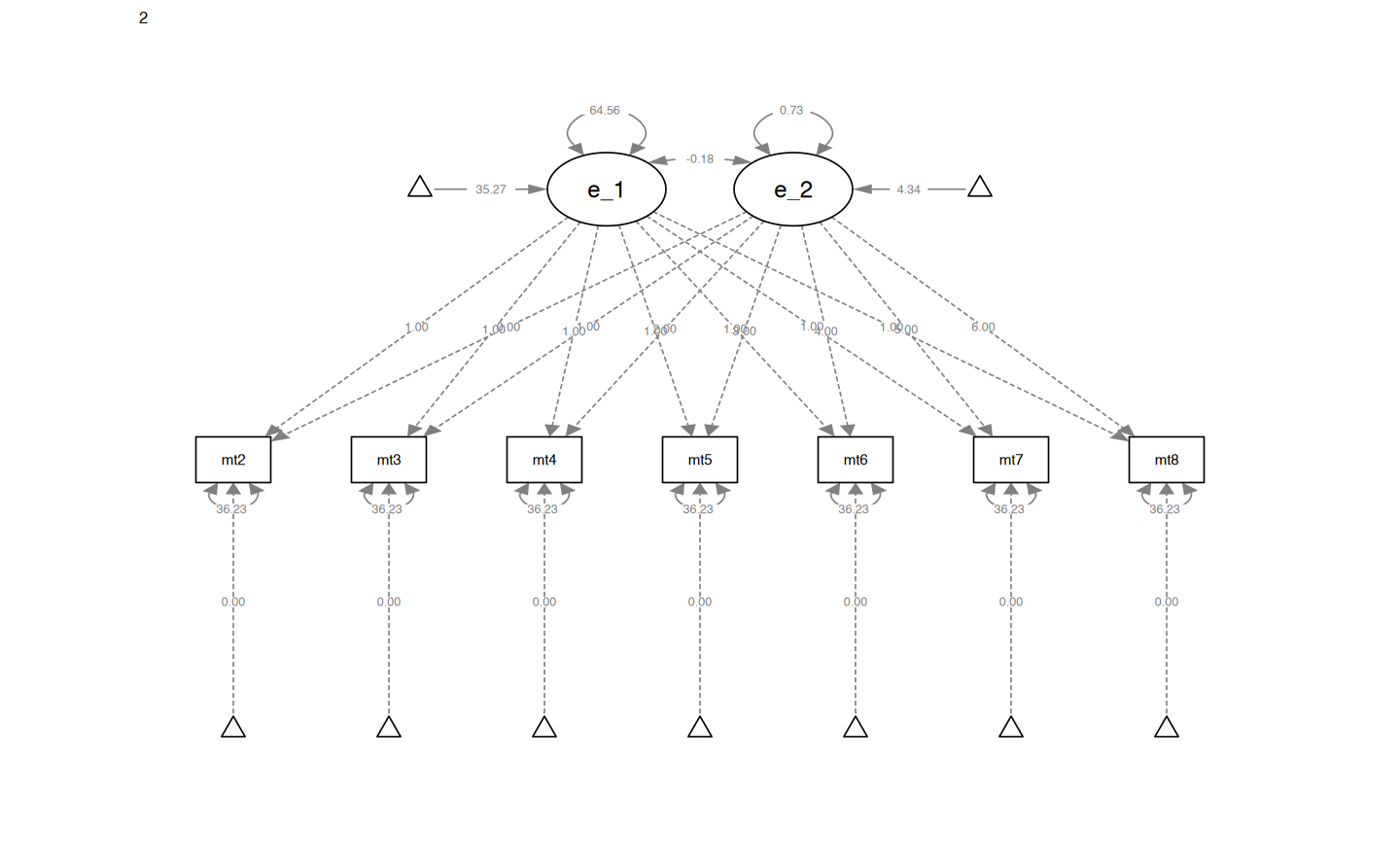
Creiamo il diagramma di percorso.
semPaths(mg_math_lavaan_fitM1, what = "path", whatLabels = "par")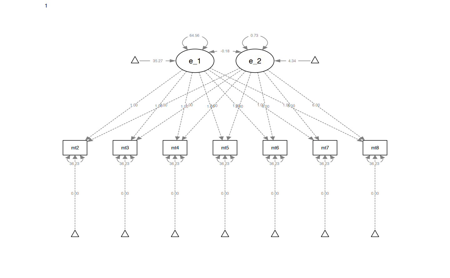
80.3 Vincoli sulle medie
Trasformiamo ora il modello restrittivo specificato in precedenza allentando via via i vincoli che abbiamo introdotto. In questo modello rendiamo possibile la differenza tra le medie nei due gruppi.
mg_math_lavaan_fitM2 <- sem(mg_math_lavaan_model,
  data = nlsy_math_wide,
  meanstructure = TRUE,
  estimator = "ML",
  missing = "fiml",
  group = "lb_wght", # to separate groups
  group.equal = c(
    "loadings", # for constraints
    # "means", commented out so can differ
    "lv.variances",
    "lv.covariances",
    "residuals"
  )
)
Esaminiamo i risultati.
summary(mg_math_lavaan_fitM2, fit.measures = TRUE) |>
    print()
lavaan 0.6-19 ended normally after 31 iterations
Estimator ML
Optimization method NLMINB
Number of model parameters 24
Number of equality constraints 16
Number of observations per group: Used Total
0 857 858
1 75 75
Number of missing patterns per group:
0 60
1 25
Model Test User Model:
Test statistic 243.910
Degrees of freedom 62
P-value (Chi-square) 0.000
Test statistic for each group:
0 191.440
1 52.470
Model Test Baseline Model:
Test statistic 887.887
Degrees of freedom 42
P-value 0.000
User Model versus Baseline Model:
Comparative Fit Index (CFI) 0.785
Tucker-Lewis Index (TLI) 0.854
Robust Comparative Fit Index (CFI) 1.000
Robust Tucker-Lewis Index (TLI) 0.326
Loglikelihood and Information Criteria:
Loglikelihood user model (H0) -7966.093
Loglikelihood unrestricted model (H1) -7844.138
Akaike (AIC) 15948.185
Bayesian (BIC) 15986.884
Sample-size adjusted Bayesian (SABIC) 15961.477
Root Mean Square Error of Approximation:
RMSEA 0.079
90 Percent confidence interval - lower 0.069
90 Percent confidence interval - upper 0.090
P-value H_0: RMSEA <= 0.050 0.000
P-value H_0: RMSEA >= 0.080 0.472
Robust RMSEA 0.000
90 Percent confidence interval - lower 0.000
90 Percent confidence interval - upper 0.000
P-value H_0: Robust RMSEA <= 0.050 1.000
P-value H_0: Robust RMSEA >= 0.080 0.000
Standardized Root Mean Square Residual:
SRMR 0.127
Parameter Estimates:
Standard errors Standard
Information Observed
Observed information based on Hessian
Group 1 [0]:
Latent Variables:
Estimate Std.Err z-value P(>|z|)
eta_1 =~
math2 1.000
math3 1.000
math4 1.000
math5 1.000
math6 1.000
math7 1.000
math8 1.000
eta_2 =~
math2 0.000
math3 1.000
math4 2.000
math5 3.000
math6 4.000
math7 5.000
math8 6.000
Covariances:
Estimate Std.Err z-value P(>|z|)
eta_1 ~~
eta_2 (.17.) -0.035 1.144 -0.031 0.975
Intercepts:
Estimate Std.Err z-value P(>|z|)
eta_1 35.488 0.369 96.080 0.000
eta_2 4.292 0.092 46.898 0.000
.math2 0.000
.math3 0.000
.math4 0.000
.math5 0.000
.math6 0.000
.math7 0.000
.math8 0.000
Variances:
Estimate Std.Err z-value P(>|z|)
eta_1 (.15.) 63.704 5.637 11.301 0.000
eta_2 (.16.) 0.699 0.325 2.147 0.032
.math2 (thet) 36.321 1.871 19.413 0.000
.math3 (thet) 36.321 1.871 19.413 0.000
.math4 (thet) 36.321 1.871 19.413 0.000
.math5 (thet) 36.321 1.871 19.413 0.000
.math6 (thet) 36.321 1.871 19.413 0.000
.math7 (thet) 36.321 1.871 19.413 0.000
.math8 (thet) 36.321 1.871 19.413 0.000
Group 2 [1]:
Latent Variables:
Estimate Std.Err z-value P(>|z|)
eta_1 =~
math2 1.000
math3 1.000
math4 1.000
math5 1.000
math6 1.000
math7 1.000
math8 1.000
eta_2 =~
math2 0.000
math3 1.000
math4 2.000
math5 3.000
math6 4.000
math7 5.000
math8 6.000
Covariances:
Estimate Std.Err z-value P(>|z|)
eta_1 ~~
eta_2 (.17.) -0.035 1.144 -0.031 0.975
Intercepts:
Estimate Std.Err z-value P(>|z|)
eta_1 32.733 1.244 26.314 0.000
eta_2 4.905 0.320 15.320 0.000
.math2 0.000
.math3 0.000
.math4 0.000
.math5 0.000
.math6 0.000
.math7 0.000
.math8 0.000
Variances:
Estimate Std.Err z-value P(>|z|)
eta_1 (.15.) 63.704 5.637 11.301 0.000
eta_2 (.16.) 0.699 0.325 2.147 0.032
.math2 (thet) 36.321 1.871 19.413 0.000
.math3 (thet) 36.321 1.871 19.413 0.000
.math4 (thet) 36.321 1.871 19.413 0.000
.math5 (thet) 36.321 1.871 19.413 0.000
.math6 (thet) 36.321 1.871 19.413 0.000
.math7 (thet) 36.321 1.871 19.413 0.000
.math8 (thet) 36.321 1.871 19.413 0.000
Eseguiamo il confronto tra i due modelli.
lavTestLRT(mg_math_lavaan_fitM1, mg_math_lavaan_fitM2) |>
    print()
Chi-Squared Difference Test

                     Df   AIC   BIC  Chisq Chisq diff    RMSEA Df diff
mg_math_lavaan_fitM2 62 15948 15987 243.91
mg_math_lavaan_fitM1 64 15949 15978 249.11     5.2005 0.058601       2
                     Pr(>Chisq)
mg_math_lavaan_fitM2
mg_math_lavaan_fitM1    0.07425 .
---
Signif. codes:  0 '***' 0.001 '**' 0.01 '*' 0.05 '.' 0.1 ' ' 1
Non vi è evidenza che consentire una differenza tra medie tra gruppi migliori l’adattamento del modello.
80.4 Vincoli sulle varianze/covarianze
Nel modello M3 consentiamo che anche le varianza e le covarianza differiscano tra gruppi, oltre alle medie.
mg_math_lavaan_fitM3 <- sem(mg_math_lavaan_model,
  data = nlsy_math_wide,
  meanstructure = TRUE,
  estimator = "ML",
  missing = "fiml",
  group = "lb_wght", # to separate groups
  group.equal = c(
    "loadings", # for constraints
    # "means", commented out so can differ
    # "lv.variances",
    # "lv.covariances",
    "residuals"
  )
)
Esaminiamo i risultati.
summary(mg_math_lavaan_fitM3, fit.measures = TRUE) |>
    print()
lavaan 0.6-19 ended normally after 57 iterations
Estimator ML
Optimization method NLMINB
Number of model parameters 24
Number of equality constraints 13
Number of observations per group: Used Total
0 857 858
1 75 75
Number of missing patterns per group:
0 60
1 25
Model Test User Model:
Test statistic 241.182
Degrees of freedom 59
P-value (Chi-square) 0.000
Test statistic for each group:
0 191.157
1 50.024
Model Test Baseline Model:
Test statistic 887.887
Degrees of freedom 42
P-value 0.000
User Model versus Baseline Model:
Comparative Fit Index (CFI) 0.785
Tucker-Lewis Index (TLI) 0.847
Robust Comparative Fit Index (CFI) 1.000
Robust Tucker-Lewis Index (TLI) 0.320
Loglikelihood and Information Criteria:
Loglikelihood user model (H0) -7964.728
Loglikelihood unrestricted model (H1) -7844.138
Akaike (AIC) 15951.457
Bayesian (BIC) 16004.668
Sample-size adjusted Bayesian (SABIC) 15969.732
Root Mean Square Error of Approximation:
RMSEA 0.081
90 Percent confidence interval - lower 0.071
90 Percent confidence interval - upper 0.092
P-value H_0: RMSEA <= 0.050 0.000
P-value H_0: RMSEA >= 0.080 0.598
Robust RMSEA 0.000
90 Percent confidence interval - lower 0.000
90 Percent confidence interval - upper 0.000
P-value H_0: Robust RMSEA <= 0.050 1.000
P-value H_0: Robust RMSEA >= 0.080 0.000
Standardized Root Mean Square Residual:
SRMR 0.124
Parameter Estimates:
Standard errors Standard
Information Observed
Observed information based on Hessian
Group 1 [0]:
Latent Variables:
Estimate Std.Err z-value P(>|z|)
eta_1 =~
math2 1.000
math3 1.000
math4 1.000
math5 1.000
math6 1.000
math7 1.000
math8 1.000
eta_2 =~
math2 0.000
math3 1.000
math4 2.000
math5 3.000
math6 4.000
math7 5.000
math8 6.000
Covariances:
Estimate Std.Err z-value P(>|z|)
eta_1 ~~
eta_2 0.243 1.147 0.212 0.832
Intercepts:
Estimate Std.Err z-value P(>|z|)
eta_1 35.485 0.365 97.271 0.000
eta_2 4.293 0.091 47.089 0.000
.math2 0.000
.math3 0.000
.math4 0.000
.math5 0.000
.math6 0.000
.math7 0.000
.math8 0.000
Variances:
Estimate Std.Err z-value P(>|z|)
eta_1 61.062 5.692 10.727 0.000
eta_2 0.663 0.326 2.033 0.042
.math2 (thet) 36.276 1.870 19.402 0.000
.math3 (thet) 36.276 1.870 19.402 0.000
.math4 (thet) 36.276 1.870 19.402 0.000
.math5 (thet) 36.276 1.870 19.402 0.000
.math6 (thet) 36.276 1.870 19.402 0.000
.math7 (thet) 36.276 1.870 19.402 0.000
.math8 (thet) 36.276 1.870 19.402 0.000
Group 2 [1]:
Latent Variables:
Estimate Std.Err z-value P(>|z|)
eta_1 =~
math2 1.000
math3 1.000
math4 1.000
math5 1.000
math6 1.000
math7 1.000
math8 1.000
eta_2 =~
math2 0.000
math3 1.000
math4 2.000
math5 3.000
math6 4.000
math7 5.000
math8 6.000
Covariances:
Estimate Std.Err z-value P(>|z|)
eta_1 ~~
eta_2 -3.801 4.912 -0.774 0.439
Intercepts:
Estimate Std.Err z-value P(>|z|)
eta_1 32.850 1.413 23.241 0.000
eta_2 4.881 0.341 14.332 0.000
.math2 0.000
.math3 0.000
.math4 0.000
.math5 0.000
.math6 0.000
.math7 0.000
.math8 0.000
Variances:
Estimate Std.Err z-value P(>|z|)
eta_1 95.283 24.221 3.934 0.000
eta_2 1.297 1.315 0.986 0.324
.math2 (thet) 36.276 1.870 19.402 0.000
.math3 (thet) 36.276 1.870 19.402 0.000
.math4 (thet) 36.276 1.870 19.402 0.000
.math5 (thet) 36.276 1.870 19.402 0.000
.math6 (thet) 36.276 1.870 19.402 0.000
.math7 (thet) 36.276 1.870 19.402 0.000
.math8 (thet) 36.276 1.870 19.402 0.000
Confrontiamo il modello M2 con il modello M3.
lavTestLRT(mg_math_lavaan_fitM2, mg_math_lavaan_fitM3) |>
    print()
Chi-Squared Difference Test

                     Df   AIC   BIC  Chisq Chisq diff RMSEA Df diff
mg_math_lavaan_fitM3 59 15952 16005 241.18
mg_math_lavaan_fitM2 62 15948 15987 243.91     2.7283     0       3
                     Pr(>Chisq)
mg_math_lavaan_fitM3
mg_math_lavaan_fitM2     0.4354
Non ci sono evidenze che una differenza nelle varianze e nelle covarianze tra gruppi migliori la bontà dell’adattamento del modello ai dati.
80.5 Vincoli sui residui
Esaminiamo ora il vincolo sulle covarianze residue. Iniziamo a specificare il modello in una nuova forma.
mg_math_lavaan_model4 <- "
  # latent variable definitions
      #intercept (note intercept is a reserved term)
      eta_1 =~ 1*math2
      eta_1 =~ 1*math3
      eta_1 =~ 1*math4
      eta_1 =~ 1*math5
      eta_1 =~ 1*math6
      eta_1 =~ 1*math7
      eta_1 =~ 1*math8

      #linear slope
      eta_2 =~ 0*math2
      eta_2 =~ 1*math3
      eta_2 =~ 2*math4
      eta_2 =~ 3*math5
      eta_2 =~ 4*math6
      eta_2 =~ 5*math7
      eta_2 =~ 6*math8

  # factor variances
      eta_1 ~~ start(60)*eta_1
      eta_2 ~~ start(.75)*eta_2

  # covariances among factors
      eta_1 ~~ eta_2

  # factor means
      eta_1 ~ start(35)*1
      eta_2 ~ start(4)*1

  # manifest variances (made equivalent by naming theta)
      math2 ~~ c(theta1,theta2)*math2
      math3 ~~ c(theta1,theta2)*math3
      math4 ~~ c(theta1,theta2)*math4
      math5 ~~ c(theta1,theta2)*math5
      math6 ~~ c(theta1,theta2)*math6
      math7 ~~ c(theta1,theta2)*math7
      math8 ~~ c(theta1,theta2)*math8
  # manifest means (fixed at zero)
      math2 ~ 0*1
      math3 ~ 0*1
      math4 ~ 0*1
      math5 ~ 0*1
      math6 ~ 0*1
      math7 ~ 0*1
      math8 ~ 0*1
" # end of model definition
Adattiamo il modello ai dati.
mg_math_lavaan_fitM4 <- sem(mg_math_lavaan_model4,
  data = nlsy_math_wide,
  meanstructure = TRUE,
  estimator = "ML",
  missing = "fiml",
  group = "lb_wght", # to separate groups
  group.equal = c("loadings")
) # for constraints
Esaminiamo i risulati.
summary(mg_math_lavaan_fitM4, fit.measures = TRUE) |>
    print()
lavaan 0.6-19 ended normally after 62 iterations
Estimator ML
Optimization method NLMINB
Number of model parameters 24
Number of equality constraints 12
Number of observations per group: Used Total
0 857 858
1 75 75
Number of missing patterns per group:
0 60
1 25
Model Test User Model:
Test statistic 237.836
Degrees of freedom 58
P-value (Chi-square) 0.000
Test statistic for each group:
0 190.833
1 47.004
Model Test Baseline Model:
Test statistic 887.887
Degrees of freedom 42
P-value 0.000
User Model versus Baseline Model:
Comparative Fit Index (CFI) 0.787
Tucker-Lewis Index (TLI) 0.846
Robust Comparative Fit Index (CFI) 1.000
Robust Tucker-Lewis Index (TLI) 0.294
Loglikelihood and Information Criteria:
Loglikelihood user model (H0) -7963.056
Loglikelihood unrestricted model (H1) -7844.138
Akaike (AIC) 15950.111
Bayesian (BIC) 16008.159
Sample-size adjusted Bayesian (SABIC) 15970.048
Root Mean Square Error of Approximation:
RMSEA 0.082
90 Percent confidence interval - lower 0.071
90 Percent confidence interval - upper 0.092
P-value H_0: RMSEA <= 0.050 0.000
P-value H_0: RMSEA >= 0.080 0.607
Robust RMSEA 0.000
90 Percent confidence interval - lower 0.000
90 Percent confidence interval - upper 0.000
P-value H_0: Robust RMSEA <= 0.050 1.000
P-value H_0: Robust RMSEA >= 0.080 0.000
Standardized Root Mean Square Residual:
SRMR 0.124
Parameter Estimates:
Standard errors Standard
Information Observed
Observed information based on Hessian
Group 1 [0]:
Latent Variables:
Estimate Std.Err z-value P(>|z|)
eta_1 =~
math2 1.000
math3 1.000
math4 1.000
math5 1.000
math6 1.000
math7 1.000
math8 1.000
eta_2 =~
math2 0.000
math3 1.000
math4 2.000
math5 3.000
math6 4.000
math7 5.000
math8 6.000
Covariances:
Estimate Std.Err z-value P(>|z|)
eta_1 ~~
eta_2 -0.063 1.161 -0.054 0.957
Intercepts:
Estimate Std.Err z-value P(>|z|)
eta_1 35.481 0.365 97.257 0.000
eta_2 4.297 0.091 47.145 0.000
.math2 0.000
.math3 0.000
.math4 0.000
.math5 0.000
.math6 0.000
.math7 0.000
.math8 0.000
Variances:
Estimate Std.Err z-value P(>|z|)
eta_1 62.287 5.728 10.873 0.000
eta_2 0.774 0.334 2.314 0.021
.math2 (tht1) 35.172 1.904 18.473 0.000
.math3 (tht1) 35.172 1.904 18.473 0.000
.math4 (tht1) 35.172 1.904 18.473 0.000
.math5 (tht1) 35.172 1.904 18.473 0.000
.math6 (tht1) 35.172 1.904 18.473 0.000
.math7 (tht1) 35.172 1.904 18.473 0.000
.math8 (tht1) 35.172 1.904 18.473 0.000
Group 2 [1]:
Latent Variables:
Estimate Std.Err z-value P(>|z|)
eta_1 =~
math2 1.000
math3 1.000
math4 1.000
math5 1.000
math6 1.000
math7 1.000
math8 1.000
eta_2 =~
math2 0.000
math3 1.000
math4 2.000
math5 3.000
math6 4.000
math7 5.000
math8 6.000
Covariances:
Estimate Std.Err z-value P(>|z|)
eta_1 ~~
eta_2 0.745 5.522 0.135 0.893
Intercepts:
Estimate Std.Err z-value P(>|z|)
eta_1 32.800 1.407 23.314 0.000
eta_2 4.873 0.341 14.298 0.000
.math2 0.000
.math3 0.000
.math4 0.000
.math5 0.000
.math6 0.000
.math7 0.000
.math8 0.000
Variances:
Estimate Std.Err z-value P(>|z|)
eta_1 79.627 25.629 3.107 0.002
eta_2 -0.157 1.477 -0.106 0.915
.math2 (tht2) 48.686 8.444 5.766 0.000
.math3 (tht2) 48.686 8.444 5.766 0.000
.math4 (tht2) 48.686 8.444 5.766 0.000
.math5 (tht2) 48.686 8.444 5.766 0.000
.math6 (tht2) 48.686 8.444 5.766 0.000
.math7 (tht2) 48.686 8.444 5.766 0.000
.math8 (tht2) 48.686 8.444 5.766 0.000
Facciamo un confronto tra la bontà di adattamento del modello M3 e del modello M4.
lavTestLRT(mg_math_lavaan_fitM3, mg_math_lavaan_fitM4) |>
    print()
Chi-Squared Difference Test

                     Df   AIC   BIC  Chisq Chisq diff    RMSEA Df diff
mg_math_lavaan_fitM4 58 15950 16008 237.84
mg_math_lavaan_fitM3 59 15952 16005 241.18     3.3457 0.070948       1
                     Pr(>Chisq)
mg_math_lavaan_fitM4
mg_math_lavaan_fitM3    0.06738 .
---
Signif. codes:  0 '***' 0.001 '**' 0.01 '*' 0.05 '.' 0.1 ' ' 1
Anche in questo caso non otteniamo un risultato che fornisce evidenza di differenze tra i due gruppi.
In sintesi, possiamo dire che le evidenze presenti suggeriscono che i modelli di crescita latente per di due gruppi hanno parametri uguali per ciò che concerne le saturazioni fattoriali, le medie, le varianze, le covarianze e i residui.
80.6 Riflessioni Conclusive
L’approccio a gruppi multipli, utilizzato per studiare le differenze interpersonali nei cambiamenti intrapersonali, è estremamente efficace. Qui ci siamo concentrati sui modelli di crescita lineare per descrivere i cambiamenti intrapersonali e le differenze interpersonali in questi cambiamenti, ma è anche possibile considerare modelli non lineari più complessi. Per esempio, in alcune situazioni, un gruppo potrebbe seguire una traiettoria di crescita lineare (ad esempio, un gruppo di controllo), mentre un altro potrebbe seguire una crescita esponenziale (ad esempio, un gruppo di intervento).
Quando consideriamo l’ipotesi che gruppi diversi di individui possano seguire traiettorie di cambiamento intrapersonale differenti, l’utilità del framework a gruppi multipli diventa ancora più evidente. Abbiamo presentato il framework a gruppi multipli come alternativa all’approccio con covarianti invarianti nel tempo, tuttavia i due approcci possono essere integrati. Come descritto nel capitolo precedente, i covarianti invarianti nel tempo sono utilizzati per spiegare le differenze interpersonali nell’intercetta e nella pendenza. Includendo i covarianti invarianti nel tempo nel framework a gruppi multipli, possiamo spiegare la variabilità nell’intercetta e nella pendenza all’interno di ciascun gruppo e testare se le relazioni tra i covarianti invarianti nel tempo e l’intercetta e la pendenza differiscono tra i gruppi.