here::here("code", "_common.R") |>
  source()

if (!requireNamespace("pacman")) install.packages("pacman")
pacman::p_load(lavaan, modelsummary)25 Punteggio totale e modello fattoriale
In questo capitolo imparerai a
- comprendere le condizioni che giustificano l’uso del punteggio totale del test.
Prerequisiti
- Leggere il capitolo 6, Factor Analysis and Principal Component Analysis, del testo Principles of psychological assessment di Petersen (2024).
Preparazione del Notebook
25.1 Introduzione
In questo capitolo affrontiamo una questione centrale nella costruzione e interpretazione dei test psicometrici: è corretto utilizzare il punteggio totale come misura del costrutto latente che il test intende rilevare?
L’uso del punteggio totale (cioè la semplice somma dei punteggi degli item) è una pratica diffusissima nella ricerca psicologica e nelle applicazioni cliniche. Tuttavia, tale uso è giustificabile solo in circostanze ben precise. Come mostrano McNeish & Wolf (2020), è necessario verificare che i dati raccolti rispettino determinate assunzioni. In caso contrario, il punteggio totale può essere una misura fuorviante del costrutto.
Per comprendere quando il punteggio totale può essere considerato una misura adeguata del costrutto latente, dobbiamo considerare il legame tra il punteggio totale e i modelli di misura fattoriali, in particolare il modello parallelo e il modello congenerico.
25.2 Punteggio totale e modello fattoriale parallelo
25.2.1 Il modello parallelo
Secondo McNeish & Wolf (2020), il punteggio totale può essere considerato una misura valida del costrutto solo se gli item soddisfano i requisiti del modello fattoriale parallelo. Questo modello implica:
- saturazioni fattoriali uguali per tutti gli item (ad esempio, tutte uguali a 1);
- varianze residue uguali tra gli item.
In termini psicometrici, questo significa assumere che ogni item contribuisce nella stessa misura alla valutazione del costrutto, e che ha lo stesso livello di “rumore” o errore.
25.2.2 Esempio: Dati di Holzinger e Swineford (1939)
McNeish & Wolf (2020) illustrano il problema usando i dati classici di Holzinger e Swineford. Gli item considerati sono:
- Paragraph comprehension
- Sentence completion
- Word definitions
- Speeded addition
- Speeded dot counting
- Discrimination between curved and straight letters
Importiamo i dati in R:
Supponiamo ora di voler stimare il costrutto sottostante utilizzando il punteggio totale:
\[ \text{Punteggio totale} = \text{Item 1 + Item 2 + Item 3 + Item 4 + Item 5 + Item 6} \]
Questo equivale ad assumere che ogni item fornisca esattamente la stessa quantità di informazione sul costrutto. Formalmente, ciò può essere espresso da un modello parallelo nel quale tutte le saturazioni fattoriali sono fissate a 1 e tutte le varianze residue sono uguali.
m_parallel <- "
  f1 =~ 1*X4 + 1*X5 + 1*X6 + 1*X7 + 1*X8 + 1*X9
  X4 ~~ theta*X4
  X5 ~~ theta*X5
  X6 ~~ theta*X6
  X7 ~~ theta*X7
  X8 ~~ theta*X8
  X9 ~~ theta*X9
"
fit_parallel <- sem(m_parallel, data = d)25.2.3 Confronto tra punteggio totale e punteggio fattoriale
Calcoliamo ora il punteggio totale e i punteggi fattoriali stimati dal modello:
d$ts <- with(d, X4 + X5 + X6 + X7 + X8 + X9)
d$scores <- as.numeric(lavPredict(fit_parallel, method="regression"))
Visualizziamo la relazione tra i due:
ggplot(d, aes(x = ts, y = scores)) + geom_point()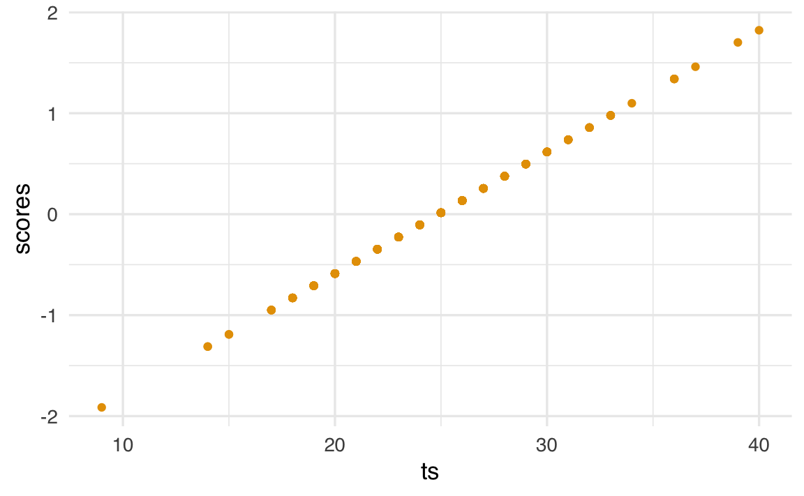
Se il modello parallelo fosse corretto, il punteggio totale e il punteggio fattoriale dovrebbero essere perfettamente correlati. Tuttavia, l’output di lavaan mostra che il modello parallelo non si adatta bene ai dati:
summary(fit_parallel, fit.measures = TRUE, standardized = TRUE)
#> lavaan 0.6-19 ended normally after 13 iterations
#>
#>   Estimator                                         ML
#>   Optimization method                           NLMINB
#>   Number of model parameters                         7
#>   Number of equality constraints                     5
#>
#>   Number of observations                           301
#>
#> Model Test User Model:
#>
#>   Test statistic                               325.899
#>   Degrees of freedom                                19
#>   P-value (Chi-square)                           0.000
#>
#> Model Test Baseline Model:
#>
#>   Test statistic                               568.519
#>   Degrees of freedom                                15
#>   P-value                                        0.000
#>
#> User Model versus Baseline Model:
#>
#>   Comparative Fit Index (CFI)                    0.446
#>   Tucker-Lewis Index (TLI)                       0.562
#>
#> Loglikelihood and Information Criteria:
#>
#>   Loglikelihood user model (H0)              -2680.931
#>   Loglikelihood unrestricted model (H1)      -2517.981
#>
#>   Akaike (AIC)                                5365.862
#>   Bayesian (BIC)                              5373.276
#>   Sample-size adjusted Bayesian (SABIC)       5366.933
#>
#> Root Mean Square Error of Approximation:
#>
#>   RMSEA                                          0.232
#>   90 Percent confidence interval - lower         0.210
#>   90 Percent confidence interval - upper         0.254
#>   P-value H_0: RMSEA <= 0.050                    0.000
#>   P-value H_0: RMSEA >= 0.080                    1.000
#>
#> Standardized Root Mean Square Residual:
#>
#>   SRMR                                           0.206
#>
#> Parameter Estimates:
#>
#>   Standard errors                             Standard
#>   Information                                 Expected
#>   Information saturated (h1) model          Structured
#>
#> Latent Variables:
#>                    Estimate  Std.Err  z-value  P(>|z|)   Std.lv  Std.all
#>   f1 =~
#>     X4                1.000                               0.633    0.551
#>     X5                1.000                               0.633    0.551
#>     X6                1.000                               0.633    0.551
#>     X7                1.000                               0.633    0.551
#>     X8                1.000                               0.633    0.551
#>     X9                1.000                               0.633    0.551
#>
#> Variances:
#>                    Estimate  Std.Err  z-value  P(>|z|)   Std.lv  Std.all
#>    .X4      (thet)    0.920    0.034   27.432    0.000    0.920    0.697
#>    .X5      (thet)    0.920    0.034   27.432    0.000    0.920    0.697
#>    .X6      (thet)    0.920    0.034   27.432    0.000    0.920    0.697
#>    .X7      (thet)    0.920    0.034   27.432    0.000    0.920    0.697
#>    .X8      (thet)    0.920    0.034   27.432    0.000    0.920    0.697
#>    .X9      (thet)    0.920    0.034   27.432    0.000    0.920    0.697
#>     f1                0.400    0.045    8.803    0.000    1.000    1.000
In questo caso, l’uso del punteggio totale non è giustificato: gli item non contribuiscono in modo uniforme alla misura del costrutto, e le ipotesi del modello parallelo non sono rispettate.
25.3 Punteggio totale e modello congenerico
25.3.1 Il modello congenerico
Il modello congenerico è una generalizzazione del modello parallelo. Qui si ammette che gli item possano avere saturazioni fattoriali differenti e varianze residue differenti. In pratica, si riconosce che alcuni item sono più informativi di altri.
m_congeneric <- "
  f1 =~ NA*X4 + X5 + X6 + X7 + X8 + X9
  f1 ~~ 1*f1
"
fit_congeneric <- sem(m_congeneric, data = d)Analizziamo le saturazioni fattoriali:
parameterEstimates(fit_congeneric, standardized = TRUE) %>%
  dplyr::filter(op == "=~") %>%
  dplyr::select(
    "Latent Factor" = lhs,
    Indicator = rhs,
    B = est,
    SE = se,
    Z = z,
    "p-value" = pvalue,
    Beta = std.all
  ) %>%
  knitr::kable(
    digits = 3, booktabs = TRUE, format = "markdown",
    caption = "Factor Loadings"
)| Latent Factor | Indicator | B | SE | Z | p-value | Beta |
|---|---|---|---|---|---|---|
| f1 | X4 | 0.963 | 0.059 | 16.274 | 0.000 | 0.824 |
| f1 | X5 | 1.121 | 0.067 | 16.835 | 0.000 | 0.846 |
| f1 | X6 | 0.894 | 0.058 | 15.450 | 0.000 | 0.792 |
| f1 | X7 | 0.195 | 0.071 | 2.767 | 0.006 | 0.170 |
| f1 | X8 | 0.185 | 0.063 | 2.938 | 0.003 | 0.180 |
| f1 | X9 | 0.278 | 0.065 | 4.245 | 0.000 | 0.258 |
Come si osserva, le saturazioni sono eterogenee. Ciò significa che il costrutto latente si riflette diversamente nei vari item. In tali casi, il punteggio totale—che attribuisce lo stesso peso a ciascun item—è una misura distorta del costrutto.
25.3.2 Confronto con i punteggi fattoriali del modello congenerico
Esaminiamo la relazione tra i punteggi fattoriali del modello congenerico e il punteggio totale del test.
d$scores_cong <- as.numeric(lavPredict(fit_congeneric, method="regression"))

d |>
  ggplot(aes(x = ts, y = scores_cong)) +
  geom_point()

cor(d$ts, d$scores_cong)^2
#> [1] 0.766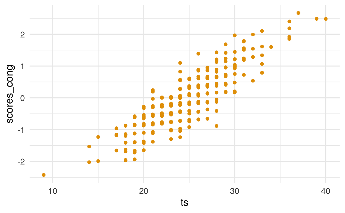
Qui il coefficiente di determinazione è circa 0.77, il che implica che due persone con lo stesso punteggio totale possono avere punteggi fattoriali molto diversi, a seconda degli item approvati. Questo è un limite importante del punteggio totale, che non tiene conto del contributo specifico di ciascun item.
Se ignoriamo le assunzioni del modello e guardiamo solo a un indice globale come l’omega, possiamo essere tratti in inganno:
psych::omega(d[, 1:6])
#> Omega
#> Call: omegah(m = m, nfactors = nfactors, fm = fm, key = key, flip = flip,
#>     digits = digits, title = title, sl = sl, labels = labels,
#>     plot = plot, n.obs = n.obs, rotate = rotate, Phi = Phi, option = option,
#>     covar = covar)
#> Alpha:                 0.72
#> G.6:                   0.76
#> Omega Hierarchical:    0.55
#> Omega H asymptotic:    0.65
#> Omega Total            0.84
#>
#> Schmid Leiman Factor loadings greater than  0.2
#>       g  F1*  F2*   F3*   h2   h2   u2   p2  com
#> X4 0.73            0.68 1.00 1.00 0.00 0.53 1.99
#> X5 0.96                 0.92 0.92 0.08 1.00 1.01
#> X6 0.69            0.22 0.54 0.54 0.46 0.90 1.22
#> X7           0.56       0.33 0.33 0.67 0.03 1.15
#> X8           0.75       0.59 0.59 0.41 0.05 1.12
#> X9 0.22      0.49       0.29 0.29 0.71 0.16 1.41
#>
#> With Sums of squares  of:
#>    g  F1*  F2*  F3*   h2
#> 2.02 0.00 1.11 0.54 2.67
#>
#> general/max  0.75   max/min =   622.1
#> mean percent general =  0.44    with sd =  0.43 and cv of  0.97
#> Explained Common Variance of the general factor =  0.55
#>
#> The degrees of freedom are 0  and the fit is  0
#> The number of observations was  301  with Chi Square =  0.03  with prob <  NA
#> The root mean square of the residuals is  0
#> The df corrected root mean square of the residuals is  NA
#>
#> Compare this with the adequacy of just a general factor and no group factors
#> The degrees of freedom for just the general factor are 9  and the fit is  0.48
#> The number of observations was  301  with Chi Square =  142.3  with prob <  3.5e-26
#> The root mean square of the residuals is  0.17
#> The df corrected root mean square of the residuals is  0.21
#>
#> RMSEA index =  0.222  and the 10 % confidence intervals are  0.191 0.255
#> BIC =  90.9
#>
#> Measures of factor score adequacy
#>                                                  g   F1*  F2*  F3*
#> Correlation of scores with factors            0.96  0.08 0.83 0.96
#> Multiple R square of scores with factors      0.93  0.01 0.68 0.91
#> Minimum correlation of factor score estimates 0.86 -0.99 0.36 0.83
#>
#>  Total, General and Subset omega for each subset
#>                                                  g  F1*  F2*  F3*
#> Omega total for total scores and subscales    0.84 0.92 0.66 0.86
#> Omega general for total scores and subscales  0.55 0.92 0.04 0.61
#> Omega group for total scores and subscales    0.27 0.00 0.61 0.25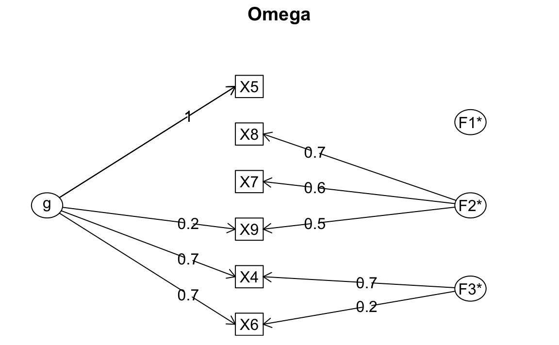
L’omega può risultare “accettabile” (Omega Total 0.84), ma ciò non garantisce che il punteggio totale sia una misura valida del costrutto.
25.4 Necessità di un modello a due fattori
I dati suggeriscono invece la presenza di due costrutti distinti. Adattiamo quindi un modello congenerico a due fattori:
m2f_cong <- "
  f1 =~ NA*X4 + X5 + X6
  f2 =~ NA*X7 + X8 + X9
  f1 ~~ 1*f1
  f2 ~~ 1*f2
  f1 ~~ f2
"
fit_2f_congeneric <- sem(m2f_cong, data = d)
summary(fit_2f_congeneric, fit.measures = TRUE, standardized = TRUE)
#> lavaan 0.6-19 ended normally after 18 iterations
#>
#>   Estimator                                         ML
#>   Optimization method                           NLMINB
#>   Number of model parameters                        13
#>
#>   Number of observations                           301
#>
#> Model Test User Model:
#>
#>   Test statistic                                14.736
#>   Degrees of freedom                                 8
#>   P-value (Chi-square)                           0.064
#>
#> Model Test Baseline Model:
#>
#>   Test statistic                               568.519
#>   Degrees of freedom                                15
#>   P-value                                        0.000
#>
#> User Model versus Baseline Model:
#>
#>   Comparative Fit Index (CFI)                    0.988
#>   Tucker-Lewis Index (TLI)                       0.977
#>
#> Loglikelihood and Information Criteria:
#>
#>   Loglikelihood user model (H0)              -2525.349
#>   Loglikelihood unrestricted model (H1)      -2517.981
#>
#>   Akaike (AIC)                                5076.698
#>   Bayesian (BIC)                              5124.891
#>   Sample-size adjusted Bayesian (SABIC)       5083.662
#>
#> Root Mean Square Error of Approximation:
#>
#>   RMSEA                                          0.053
#>   90 Percent confidence interval - lower         0.000
#>   90 Percent confidence interval - upper         0.095
#>   P-value H_0: RMSEA <= 0.050                    0.402
#>   P-value H_0: RMSEA >= 0.080                    0.159
#>
#> Standardized Root Mean Square Residual:
#>
#>   SRMR                                           0.035
#>
#> Parameter Estimates:
#>
#>   Standard errors                             Standard
#>   Information                                 Expected
#>   Information saturated (h1) model          Structured
#>
#> Latent Variables:
#>                    Estimate  Std.Err  z-value  P(>|z|)   Std.lv  Std.all
#>   f1 =~
#>     X4                0.965    0.059   16.296    0.000    0.965    0.826
#>     X5                1.123    0.067   16.845    0.000    1.123    0.847
#>     X6                0.895    0.058   15.465    0.000    0.895    0.793
#>   f2 =~
#>     X7                0.659    0.080    8.218    0.000    0.659    0.575
#>     X8                0.733    0.077    9.532    0.000    0.733    0.712
#>     X9                0.599    0.075    8.025    0.000    0.599    0.557
#>
#> Covariances:
#>                    Estimate  Std.Err  z-value  P(>|z|)   Std.lv  Std.all
#>   f1 ~~
#>     f2                0.275    0.072    3.813    0.000    0.275    0.275
#>
#> Variances:
#>                    Estimate  Std.Err  z-value  P(>|z|)   Std.lv  Std.all
#>     f1                1.000                               1.000    1.000
#>     f2                1.000                               1.000    1.000
#>    .X4                0.433    0.056    7.679    0.000    0.433    0.318
#>    .X5                0.496    0.072    6.892    0.000    0.496    0.282
#>    .X6                0.472    0.054    8.732    0.000    0.472    0.371
#>    .X7                0.881    0.100    8.807    0.000    0.881    0.670
#>    .X8                0.521    0.094    5.534    0.000    0.521    0.492
#>    .X9                0.798    0.087    9.162    0.000    0.798    0.689
Il modello mostra un buon adattamento. In questo scenario, il punteggio totale aggrega item che misurano costrutti diversi, perdendo così validità come indicatore di un singolo costrutto.
25.5 Conclusione
L’uso del punteggio totale come stima del costrutto latente è una semplificazione che deve essere giustificata empiricamente:
- é giustificato solo se il modello parallelo è supportato dai dati;
- nel caso in cui gli item abbiano saturazioni diverse (modello congenerico), il punteggio totale perde validità;
- se esistono più costrutti latenti, l’uso del punteggio totale può introdurre errori sistematici.
In sintesi: prima di usare o interpretare un punteggio totale, è essenziale testare il modello fattoriale sottostante. I punteggi totali, per quanto comodi, possono essere ingannevoli (McNeish & Wolf, 2020).
25.6 Session Info
sessionInfo()
#> R version 4.4.2 (2024-10-31)
#> Platform: aarch64-apple-darwin20
#> Running under: macOS Sequoia 15.3.2
#>
#> Matrix products: default
#> BLAS:   /Library/Frameworks/R.framework/Versions/4.4-arm64/Resources/lib/libRblas.0.dylib
#> LAPACK: /Library/Frameworks/R.framework/Versions/4.4-arm64/Resources/lib/libRlapack.dylib;  LAPACK version 3.12.0
#>
#> locale:
#> [1] C/UTF-8/C/C/C/C
#>
#> time zone: Europe/Rome
#> tzcode source: internal
#>
#> attached base packages:
#> [1] stats     graphics  grDevices utils     datasets  methods   base
#>
#> other attached packages:
#>  [1] modelsummary_2.3.0 ggokabeito_0.1.0   see_0.11.0
#>  [4] MASS_7.3-65        viridis_0.6.5      viridisLite_0.4.2
#>  [7] ggpubr_0.6.0       ggExtra_0.10.1     gridExtra_2.3
#> [10] patchwork_1.3.0    bayesplot_1.11.1   semTools_0.5-6
#> [13] semPlot_1.1.6      lavaan_0.6-19      psych_2.4.12
#> [16] scales_1.3.0       markdown_1.13      knitr_1.50
#> [19] lubridate_1.9.4    forcats_1.0.0      stringr_1.5.1
#> [22] dplyr_1.1.4        purrr_1.0.4        readr_2.1.5
#> [25] tidyr_1.3.1        tibble_3.2.1       ggplot2_3.5.1
#> [28] tidyverse_2.0.0    here_1.0.1
#>
#> loaded via a namespace (and not attached):
#>   [1] rstudioapi_0.17.1    jsonlite_1.9.1       magrittr_2.0.3
#>   [4] TH.data_1.1-3        estimability_1.5.1   farver_2.1.2
#>   [7] nloptr_2.2.1         rmarkdown_2.29       vctrs_0.6.5
#>  [10] minqa_1.2.8          base64enc_0.1-3      rstatix_0.7.2
#>  [13] htmltools_0.5.8.1    broom_1.0.7          Formula_1.2-5
#>  [16] htmlwidgets_1.6.4    plyr_1.8.9           sandwich_3.1-1
#>  [19] rio_1.2.3            emmeans_1.10.7       zoo_1.8-13
#>  [22] igraph_2.1.4         mime_0.13            lifecycle_1.0.4
#>  [25] pkgconfig_2.0.3      Matrix_1.7-3         R6_2.6.1
#>  [28] fastmap_1.2.0        rbibutils_2.3        shiny_1.10.0
#>  [31] digest_0.6.37        OpenMx_2.21.13       fdrtool_1.2.18
#>  [34] colorspace_2.1-1     rprojroot_2.0.4      Hmisc_5.2-3
#>  [37] labeling_0.4.3       timechange_0.3.0     abind_1.4-8
#>  [40] compiler_4.4.2       withr_3.0.2          glasso_1.11
#>  [43] htmlTable_2.4.3      backports_1.5.0      carData_3.0-5
#>  [46] R.utils_2.13.0       ggsignif_0.6.4       GPArotation_2024.3-1
#>  [49] corpcor_1.6.10       gtools_3.9.5         tools_4.4.2
#>  [52] pbivnorm_0.6.0       foreign_0.8-88       zip_2.3.2
#>  [55] httpuv_1.6.15        nnet_7.3-20          R.oo_1.27.0
#>  [58] glue_1.8.0           quadprog_1.5-8       nlme_3.1-167
#>  [61] promises_1.3.2       lisrelToR_0.3        grid_4.4.2
#>  [64] checkmate_2.3.2      cluster_2.1.8.1      reshape2_1.4.4
#>  [67] generics_0.1.3       gtable_0.3.6         tzdb_0.5.0
#>  [70] R.methodsS3_1.8.2    data.table_1.17.0    hms_1.1.3
#>  [73] car_3.1-3            tables_0.9.31        sem_3.1-16
#>  [76] pillar_1.10.1        rockchalk_1.8.157    later_1.4.1
#>  [79] splines_4.4.2        lattice_0.22-6       survival_3.8-3
#>  [82] kutils_1.73          tidyselect_1.2.1     miniUI_0.1.1.1
#>  [85] pbapply_1.7-2        reformulas_0.4.0     stats4_4.4.2
#>  [88] xfun_0.51            qgraph_1.9.8         arm_1.14-4
#>  [91] stringi_1.8.4        yaml_2.3.10          pacman_0.5.1
#>  [94] boot_1.3-31          evaluate_1.0.3       codetools_0.2-20
#>  [97] mi_1.1               cli_3.6.4            RcppParallel_5.1.10
#> [100] rpart_4.1.24         xtable_1.8-4         Rdpack_2.6.3
#> [103] munsell_0.5.1        Rcpp_1.0.14          coda_0.19-4.1
#> [106] png_0.1-8            XML_3.99-0.18        parallel_4.4.2
#> [109] jpeg_0.1-10          lme4_1.1-36          mvtnorm_1.3-3
#> [112] openxlsx_4.2.8       rlang_1.1.5          multcomp_1.4-28
#> [115] mnormt_2.1.1