46 ✏️ Esercizi

source("../_common.R")
suppressPackageStartupMessages({
    library("lavaan")
    library("semTools")
})
set.seed(42)

E1. Si ripeta l’esercizio che abbiamo svolto in precedenza usando l’analisi fattoriale esplorativa, questa volta usando la CFA in lavaan. I dati sono forniti da Brown (2015) e riguardano a otto misure di personalità raccolte su un campione di 250 pazienti che hanno concluso un programma di psicoterapia:

anxiety (N1),
hostility (N2),
depression (N3),
self-consciousness (N4),
warmth (E1),
gregariousness (E2),
assertiveness (E3),
positive emotions (E4).

varnames <- c("N1", "N2", "N3", "N4", "E1", "E2", "E3", "E4")
sds <- "5.7  5.6  6.4  5.7  6.0  6.2  5.7  5.6"

cors <- "
 1.000
 0.767  1.000
 0.731  0.709  1.000
 0.778  0.738  0.762  1.000
-0.351  -0.302  -0.356  -0.318  1.000
-0.316  -0.280  -0.300  -0.267  0.675  1.000
-0.296  -0.289  -0.297  -0.296  0.634  0.651  1.000
-0.282  -0.254  -0.292  -0.245  0.534  0.593  0.566  1.000"

psychot_cor_mat <- getCov(cors, names = varnames)
n <- 250

Il modello con due fattori ortogonali può essere adattato ai dati nel modo seguente.

cfa_mod <- "
  N =~ N1 + N2 + N3 + N4
  E =~ E1 + E2 + E3 + E4
"

fit_cfa <- lavaan::cfa(
    cfa_mod,
    sample.cov = psychot_cor_mat,
    sample.nobs = n,
    orthogonal = TRUE,
    std.lv = TRUE
)

semPlot::semPaths(fit_cfa,
    what = "col", whatLabels = "par", style = "mx", 
    layout = "tree2", nCharNodes = 7,
    shapeMan = "rectangle", sizeMan = 8, sizeMan2 = 5
)

Esaminiamo le saturazioni fattoriali:

parameterEstimates(fit_cfa, standardized = TRUE) %>%
    dplyr::filter(op == "=~") %>%
    dplyr::select(
        "Latent Factor" = lhs,
        Indicator = rhs,
        B = est,
        SE = se,
        Z = z,
        "p-value" = pvalue,
        Beta = std.all
    ) %>%
    knitr::kable(
        digits = 3, booktabs = TRUE, format = "markdown",
        caption = "Factor Loadings"
    )



Table: Factor Loadings

|Latent Factor |Indicator |     B|    SE|      Z| p-value|  Beta|
|:-------------|:---------|-----:|-----:|------:|-------:|-----:|
|N             |N1        | 0.882| 0.051| 17.422|       0| 0.884|
|N             |N2        | 0.847| 0.052| 16.340|       0| 0.849|
|N             |N3        | 0.840| 0.052| 16.134|       0| 0.842|
|N             |N4        | 0.882| 0.051| 17.432|       0| 0.884|
|E             |E1        | 0.795| 0.056| 14.276|       0| 0.796|
|E             |E2        | 0.838| 0.054| 15.369|       0| 0.839|
|E             |E3        | 0.788| 0.056| 14.097|       0| 0.789|
|E             |E4        | 0.697| 0.058| 11.942|       0| 0.699|

Il risultato sembra sensato: le saturazioni su ciascun fattore sono molto alte. Tuttavia, la matrice delle correlazioni residue

cor_table <- residuals(fit_cfa, type = "cor")$cov
knitr::kable(
    cor_table,
    digits = 3,
    format = "markdown",
    booktabs = TRUE
)



|   |     N1|     N2|     N3|     N4|     E1|     E2|     E3|     E4|
|:--|------:|------:|------:|------:|------:|------:|------:|------:|
|N1 |  0.000|  0.017| -0.013| -0.003| -0.351| -0.316| -0.296| -0.282|
|N2 |  0.017|  0.000| -0.006| -0.012| -0.302| -0.280| -0.289| -0.254|
|N3 | -0.013| -0.006|  0.000|  0.018| -0.356| -0.300| -0.297| -0.292|
|N4 | -0.003| -0.012|  0.018|  0.000| -0.318| -0.267| -0.296| -0.245|
|E1 | -0.351| -0.302| -0.356| -0.318|  0.000|  0.007|  0.006| -0.022|
|E2 | -0.316| -0.280| -0.300| -0.267|  0.007|  0.000| -0.011|  0.007|
|E3 | -0.296| -0.289| -0.297| -0.296|  0.006| -0.011|  0.000|  0.015|
|E4 | -0.282| -0.254| -0.292| -0.245| -0.022|  0.007|  0.015|  0.000|

rivela che il modello ipotizzato dall’analisi fattoriale confermativa non è adeguato.

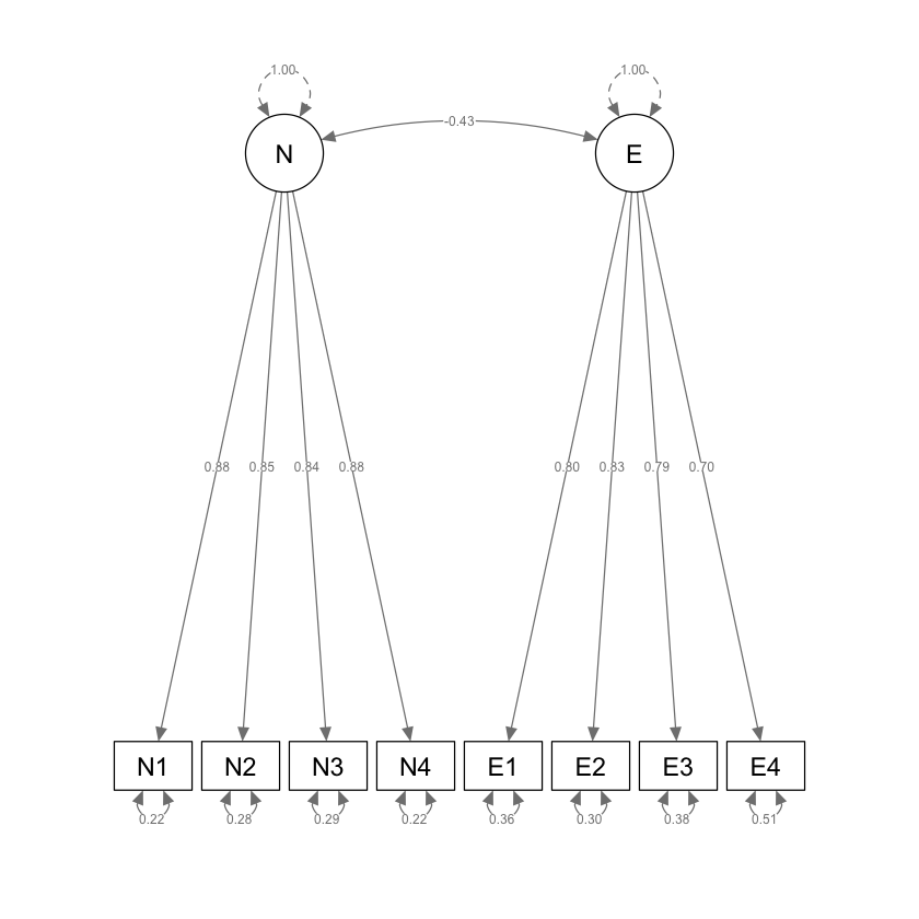
fit2_cfa <- lavaan::cfa(
    cfa_mod,
    sample.cov = psychot_cor_mat,
    sample.nobs = n,
    orthogonal = FALSE,
    std.lv = TRUE
)

semPlot::semPaths(fit2_cfa,
    what = "col", whatLabels = "par", style = "mx", 
    layout = "tree2", nCharNodes = 7,
    shapeMan = "rectangle", sizeMan = 8, sizeMan2 = 5
)

Esaminiamo le saturazioni fattoriali.

parameterEstimates(fit2_cfa, standardized = TRUE) %>%
    dplyr::filter(op == "=~") %>%
    dplyr::select(
        "Latent Factor" = lhs,
        Indicator = rhs,
        B = est,
        SE = se,
        Z = z,
        "p-value" = pvalue,
        Beta = std.all
    ) %>%
    knitr::kable(
        digits = 3, booktabs = TRUE, format = "markdown",
        caption = "Factor Loadings"
    )



Table: Factor Loadings

|Latent Factor |Indicator |     B|    SE|      Z| p-value|  Beta|
|:-------------|:---------|-----:|-----:|------:|-------:|-----:|
|N             |N1        | 0.883| 0.051| 17.472|       0| 0.885|
|N             |N2        | 0.847| 0.052| 16.337|       0| 0.849|
|N             |N3        | 0.842| 0.052| 16.190|       0| 0.844|
|N             |N4        | 0.880| 0.051| 17.381|       0| 0.882|
|E             |E1        | 0.800| 0.055| 14.465|       0| 0.802|
|E             |E2        | 0.832| 0.054| 15.294|       0| 0.834|
|E             |E3        | 0.788| 0.056| 14.150|       0| 0.789|
|E             |E4        | 0.698| 0.058| 11.974|       0| 0.699|

Esaminiamo i residui.

cor_table <- residuals(fit2_cfa, type = "cor")$cov
knitr::kable(
    cor_table,
    digits = 3,
    format = "markdown",
    booktabs = TRUE
)



|   |     N1|     N2|     N3|     N4|     E1|     E2|     E3|     E4|
|:--|------:|------:|------:|------:|------:|------:|------:|------:|
|N1 |  0.000|  0.016| -0.015| -0.002| -0.042|  0.005|  0.008| -0.013|
|N2 |  0.016|  0.000| -0.007| -0.010| -0.006|  0.028|  0.002|  0.004|
|N3 | -0.015| -0.007|  0.000|  0.018| -0.062|  0.006| -0.007| -0.035|
|N4 | -0.002| -0.010|  0.018|  0.000| -0.010|  0.053|  0.007|  0.023|
|E1 | -0.042| -0.006| -0.062| -0.010|  0.000|  0.006|  0.001| -0.027|
|E2 |  0.005|  0.028|  0.006|  0.053|  0.006|  0.000| -0.007|  0.010|
|E3 |  0.008|  0.002| -0.007|  0.007|  0.001| -0.007|  0.000|  0.014|
|E4 | -0.013|  0.004| -0.035|  0.023| -0.027|  0.010|  0.014|  0.000|

Sistemiamo le saturazioni fattoriali in una matrice 8 \(\times\) 2:

lambda <- inspect(fit2_cfa, what = "std")$lambda
lambda

A lavaan.matrix: 8 x 2 of type dbl
	N	E
N1	0.8848214	0.0000000
N2	0.8485128	0.0000000
N3	0.8436432	0.0000000
N4	0.8819736	0.0000000
E1	0.0000000	0.8018485
E2	0.0000000	0.8337599
E3	0.0000000	0.7894530
E4	0.0000000	0.6990366

Otteniamo la matrice di intercorrelazoni fattoriali.

Phi <- inspect(fit2_cfa, what = "std")$psi
Phi

A lavaan.matrix.symmetric: 2 x 2 of type dbl
	N	E
N	1.000000	-0.434962
E	-0.434962	1.000000

Otteniamo la matrice di varianze residue.

Psi <- inspect(fit2_cfa, what = "std")$theta
Psi

A lavaan.matrix.symmetric: 8 x 8 of type dbl
	N1	N2	N3	N4	E1	E2	E3	E4
N1	0.217091	0.0000000	0.0000000	0.0000000	0.000000	0.0000000	0.000000	0.0000000
N2	0.000000	0.2800261	0.0000000	0.0000000	0.000000	0.0000000	0.000000	0.0000000
N3	0.000000	0.0000000	0.2882661	0.0000000	0.000000	0.0000000	0.000000	0.0000000
N4	0.000000	0.0000000	0.0000000	0.2221225	0.000000	0.0000000	0.000000	0.0000000
E1	0.000000	0.0000000	0.0000000	0.0000000	0.357039	0.0000000	0.000000	0.0000000
E2	0.000000	0.0000000	0.0000000	0.0000000	0.000000	0.3048445	0.000000	0.0000000
E3	0.000000	0.0000000	0.0000000	0.0000000	0.000000	0.0000000	0.376764	0.0000000
E4	0.000000	0.0000000	0.0000000	0.0000000	0.000000	0.0000000	0.000000	0.5113478

Mediante i parametri del modello la matrice di correlazione si riproduce nel modo seguente:

\[ \boldsymbol{\Sigma} =\boldsymbol{\Lambda} \boldsymbol{\Phi} \boldsymbol{\Lambda}^{\mathsf{T}} + \boldsymbol{\Psi}. \]

In \(\textsf{R}\) scriviamo:

R_hat <- lambda %*% Phi %*% t(lambda) + Psi
R_hat %>%
    round(3)

A lavaan.matrix.symmetric: 8 x 8 of type dbl
	N1	N2	N3	N4	E1	E2	E3	E4
N1	1.000	0.751	0.746	0.780	-0.309	-0.321	-0.304	-0.269
N2	0.751	1.000	0.716	0.748	-0.296	-0.308	-0.291	-0.258
N3	0.746	0.716	1.000	0.744	-0.294	-0.306	-0.290	-0.257
N4	0.780	0.748	0.744	1.000	-0.308	-0.320	-0.303	-0.268
E1	-0.309	-0.296	-0.294	-0.308	1.000	0.669	0.633	0.561
E2	-0.321	-0.308	-0.306	-0.320	0.669	1.000	0.658	0.583
E3	-0.304	-0.291	-0.290	-0.303	0.633	0.658	1.000	0.552
E4	-0.269	-0.258	-0.257	-0.268	0.561	0.583	0.552	1.000

Le correlazioni residue sono:

(psychot_cor_mat - R_hat) %>%
    round(3)

A lavaan.matrix.symmetric: 8 x 8 of type dbl
	N1	N2	N3	N4	E1	E2	E3	E4
N1	0.000	0.016	-0.015	-0.002	-0.042	0.005	0.008	-0.013
N2	0.016	0.000	-0.007	-0.010	-0.006	0.028	0.002	0.004
N3	-0.015	-0.007	0.000	0.018	-0.062	0.006	-0.007	-0.035
N4	-0.002	-0.010	0.018	0.000	-0.010	0.053	0.007	0.023
E1	-0.042	-0.006	-0.062	-0.010	0.000	0.006	0.001	-0.027
E2	0.005	0.028	0.006	0.053	0.006	0.000	-0.007	0.010
E3	0.008	0.002	-0.007	0.007	0.001	-0.007	0.000	0.014
E4	-0.013	0.004	-0.035	0.023	-0.027	0.010	0.014	0.000

Calcoliamo la correlazione predetta dal modello tra le variabili \(Y_1\) e \(Y_2\):

lambda[1, 1] * lambda[2, 1] + lambda[1, 2] * lambda[2, 2] +
    lambda[1, 1] * lambda[2, 2] * Phi[1, 2] +
    lambda[1, 2] * lambda[2, 1] * Phi[1, 2]

0.750782309575684

Questo risultato è molto simile al valore contenuto dell’elemento (1, 2) della matrice di correlazioni osservate:

psychot_cor_mat[1, 2]

0.767

Usando le funzonalità di lavaan la matrice di correlazione predetta si ottiene con:

fitted(fit2_cfa)$cov |>
    print()

       N1     N2     N3     N4     E1     E2     E3     E4
N1  0.996                                                 
N2  0.748  0.996                                          
N3  0.743  0.713  0.996                                   
N4  0.777  0.745  0.741  0.996                            
E1 -0.307 -0.295 -0.293 -0.306  0.996                     
E2 -0.320 -0.306 -0.305 -0.319  0.666  0.996              
E3 -0.303 -0.290 -0.289 -0.302  0.630  0.656  0.996       
E4 -0.268 -0.257 -0.255 -0.267  0.558  0.580  0.550  0.996

La matrice dei residui è

resid(fit2_cfa)$cov |>
    print()

       N1     N2     N3     N4     E1     E2     E3     E4
N1  0.000                                                 
N2  0.016  0.000                                          
N3 -0.015 -0.007  0.000                                   
N4 -0.002 -0.010  0.018  0.000                            
E1 -0.042 -0.006 -0.062 -0.010  0.000                     
E2  0.005  0.028  0.006  0.053  0.006  0.000              
E3  0.008  0.002 -0.007  0.007  0.001 -0.007  0.000       
E4 -0.013  0.004 -0.035  0.023 -0.026  0.010  0.014  0.000

La matrice dei residui standardizzati è

resid(fit2_cfa, type = "standardized")$cov |>
    print()

       N1     N2     N3     N4     E1     E2     E3     E4
N1  0.000                                                 
N2  1.674  0.000                                          
N3 -1.769 -0.569  0.000                                   
N4 -0.350 -1.152  1.746  0.000                            
E1 -1.214 -0.161 -1.646 -0.294  0.000                     
E2  0.154  0.794  0.168  1.626  0.637  0.000              
E3  0.219  0.062 -0.191  0.193  0.075 -0.693  0.000       
E4 -0.314  0.092 -0.824  0.552 -1.481  0.624  0.690  0.000

I valori precedenti possono essere considerati come punti z, dove i valori con un valore assoluto maggiore di 2 possono essere ritenuti problematici. Tuttavia, è importante considerare che in questo modo si stanno eseguendo molteplici confronti, pertanto, si dovrebbe considerare l’opportunità di applicare una qualche forma di correzione per i confronti multipli.

E2. Si utilizzino i dati dass21.txt che corrispondono alla somministrazione del test DASS-21 a 334 partecipanti. Lo schema di codifica si può trovare seguendo questo link. Si adatti ai dati un modello a tre fattori usando l’analisi fattoriale esplorativa con la funzione lavaan::efa(). Usando le saturazioni fattoriali e la matrice di inter-correlazioni fattoriali, si trovi la matrice di correlazioni riprodotta dal modello. Senza usare l’albebra matriciale, si trovi la correlazione predetta tra gli indicatori DASS-1 e DASS-2.