85. Modello LCS bivariato#
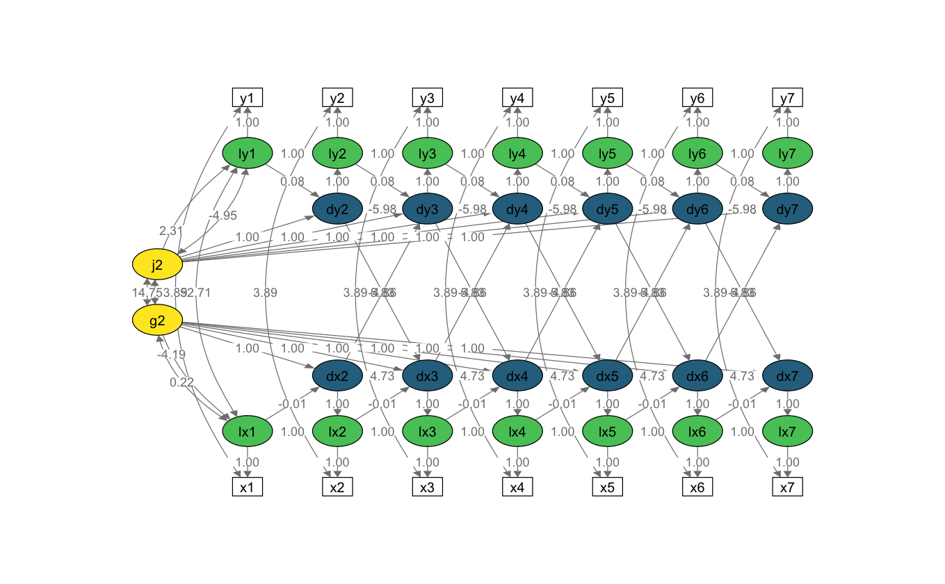
I modelli LCSM sono stati sviluppati principalmente per studiare le associazioni sequenziali nel tempo tra due o più processi che cambiano nel tempo. In altre parole, le equazioni di cambiamento latente possono essere estese per includere effetti derivanti da variabili aggiuntive per modellare congiuntamente processi multipli di sviluppo in corso (McArdle, 2001; McArdle & Hamagami, 2001). Considereremo qui un modello LCS bivariato con parametri di accoppiamento cambiamento-cambiamento ritardati. Il seguene path diagram è fornito da Wiedemann et al. [WTKovsirE22].
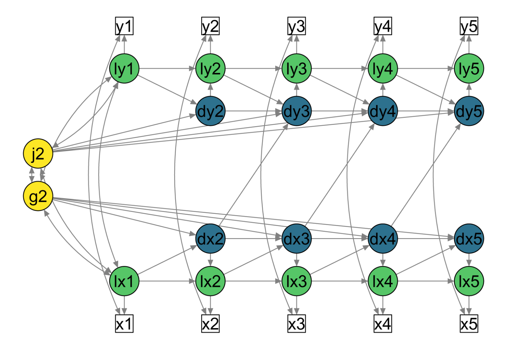
Fig. 85.1 Diagramma di percorso semplificato per un modello LCS bivariato con parametri di accoppiamento cambiamento-cambiamento ritardati (ad esempio, da dx2 a dy3). Quadrati bianchi = variabili osservate; cerchi verdi = punteggi veri latenti (prefisso ‘l’); cerchi blu = punteggi di cambiamento latenti (prefisso ‘d’); cerchi gialli = fattori di cambiamento latente costanti. Frecce direzionali = Regressioni; frecce bidirezionali = covarianze. I punteggi unici (\(ux_t\) e \(uy_t\)) e le varianze uniche (\(σ^2_{ux}\) e \(σ^2_{uy}\)) non sono mostrati in questa figura per semplicità.#
Come in precedenza per il caso del modello univariato, il modello LCSM bivariato include, per ciascuna di due variabili misurate nel tempo, un fattore di cambiamento costante (alpha_constant), un fattore di cambiamento proporzionale (beta) e l’autoregressione dei punteggi di cambiamento (phi). L’aspetto nuovo riguarda i parametri di “accoppiamento”. Per i modelli LCSM bivariati, tali parametri modellano le interazioni tra le variabili \(X\) e \(Y\). I test su tali parametri consentono di affrontare la seguente domanda della ricerca: le variazioni della variabile Y al momento (t) sono determinate dalle variazioni della variabile X al momento precedente (t-1)? E viceversa. Oppure tutte e due le condizioni insieme. I test statistici sui parametri di accoppiamento consentono di rispondere alle domande precedenti.
85.1. Illustrazione#
Per illustrare l’adattamento e l’interpretazione dei modelli LCS bivariati, analizziamo i dati longitudinali di matematica che sono stati utilizzati nel Capitolo 17 di [GRE16]. I dati longitudinali di matematica sono stati raccolti dall’NLSY-CYA (Center for Human Resource Research, 2009) e i punteggi di matematica provengono dal PIAT (Dunn & Markwardt, 1970). Vengono anche misurati i punteggi di comprensione nella lettura dal secondo all’ottavo grado scolastico. Il grado scolastico al momento del test viene utilizzato come metrica temporale e varia dalla seconda elementare (grado 2) alla terza media (grado 8).
Leggiamo i pacchetti necessari.
source("../_common.R")
suppressPackageStartupMessages({
    library("lavaan")
    library("semPlot")
    library("patchwork")
    library("psych")
    library("DT")
    library("kableExtra")
    library("lme4")
    library("lcsm")
    library("tidyr")
    library("stringr")
})
set.seed(12345)
Importiamo i dati in R utilizzando un file messo a disposizione dagli autori.
nlsy_multi_data <- read.table(file = "../data/nlsy_math_hyp_wide_R.dat", na.strings = ".")
names(nlsy_multi_data) <- c(
    "id", "female", "lb_wght", "anti_k1",
    "math2", "math3", "math4", "math5", "math6", "math7", "math8",
    "comp2", "comp3", "comp4", "comp5", "comp6", "comp7", "comp8",
    "rec2", "rec3", "rec4", "rec5", "rec6", "rec7", "rec8",
    "bpi2", "bpi3", "bpi4", "bpi5", "bpi6", "bpi7", "bpi8",
    "asl2", "asl3", "asl4", "asl5", "asl6", "asl7", "asl8",
    "ax2", "ax3", "ax4", "ax5", "ax6", "ax7", "ax8",
    "hds2", "hds3", "hds4", "hds5", "hds6", "hds7", "hds8",
    "hyp2", "hyp3", "hyp4", "hyp5", "hyp6", "hyp7", "hyp8",
    "dpn2", "dpn3", "dpn4", "dpn5", "dpn6", "dpn7", "dpn8",
    "wdn2", "wdn3", "wdn4", "wdn5", "wdn6", "wdn7", "wdn8",
    "age2", "age3", "age4", "age5", "age6", "age7", "age8",
    "men2", "men3", "men4", "men5", "men6", "men7", "men8",
    "spring2", "spring3", "spring4", "spring5", "spring6", "spring7", "spring8",
    "anti2", "anti3", "anti4", "anti5", "anti6", "anti7", "anti8"
)
Definiamo due vettori che serviranno per codificare le variabili math e rec.
x_var_list <- paste0("math", 2:8)
y_var_list <- paste0("rec", 2:8)
Estraiamo dal DataFrame originale solo le variabili relative alla matematica e alla capacità di lettura, oltre alla variabile id.
nlsy_multi_data <- nlsy_multi_data[, c("id", x_var_list, y_var_list)]
glimpse(nlsy_multi_data)
Rows: 933
Columns: 15
$ id    <int> 201, 303, 2702, 4303, 5002, 5005, 5701, 6102, 6801, 6802, 6803, …
$ math2 <int> NA, 26, 56, NA, NA, 35, NA, NA, NA, NA, NA, 35, NA, NA, NA, NA, …
$ math3 <int> 38, NA, NA, 41, NA, NA, 62, NA, 54, 55, 57, NA, 34, NA, 54, 66, …
$ math4 <int> NA, NA, 58, 58, 46, 50, 61, 55, NA, NA, NA, 59, 50, 48, NA, NA, …
$ math5 <int> 55, 33, NA, NA, NA, NA, NA, 67, 62, 66, 70, NA, NA, NA, NA, 65, …
$ math6 <int> NA, NA, NA, NA, 54, 60, NA, NA, NA, NA, NA, NA, NA, NA, 64, NA, …
$ math7 <int> NA, NA, NA, NA, NA, NA, NA, 81, 66, 68, NA, NA, NA, NA, 63, NA, …
$ math8 <int> NA, NA, 80, NA, 66, 59, NA, NA, NA, NA, NA, NA, NA, NA, NA, NA, …
$ rec2  <int> NA, 26, 33, NA, NA, 47, NA, NA, NA, NA, NA, 33, NA, NA, NA, NA, …
$ rec3  <int> 35, NA, NA, 34, NA, NA, 64, NA, 53, 66, 68, NA, 49, NA, 54, 55, …
$ rec4  <int> NA, NA, 50, 43, 46, 67, 70, 50, NA, NA, NA, 63, 53, 37, NA, NA, …
$ rec5  <int> 52, 35, NA, NA, NA, NA, NA, 69, 76, 66, 70, NA, NA, NA, NA, 78, …
$ rec6  <int> NA, NA, NA, NA, 70, 75, NA, NA, NA, NA, NA, NA, NA, NA, 71, NA, …
$ rec7  <int> NA, NA, NA, NA, NA, NA, NA, 71, 64, 75, NA, NA, NA, NA, 74, NA, …
$ rec8  <int> NA, NA, 66, NA, 77, 78, NA, NA, NA, NA, NA, NA, NA, NA, NA, NA, …
Esaminiamo le statistiche descrittive.
psych::describe(nlsy_multi_data)
| vars | n | mean | sd | median | trimmed | mad | min | max | range | skew | kurtosis | se | |
|---|---|---|---|---|---|---|---|---|---|---|---|---|---|
| <int> | <dbl> | <dbl> | <dbl> | <dbl> | <dbl> | <dbl> | <dbl> | <dbl> | <dbl> | <dbl> | <dbl> | <dbl> | |
| id | 1 | 933 | 532334.89711 | 3.280208e+05 | 506602.0 | 520130.77108 | 391999.4400 | 201 | 1256601 | 1256400 | 0.28416593 | -0.90788724 | 1.073892e+04 |
| math2 | 2 | 335 | 32.60896 | 1.028600e+01 | 32.0 | 32.27509 | 10.3782 | 12 | 60 | 48 | 0.26866808 | -0.46001296 | 5.619840e-01 |
| math3 | 3 | 431 | 39.88399 | 1.029949e+01 | 41.0 | 39.88406 | 10.3782 | 13 | 67 | 54 | -0.05209289 | -0.32591683 | 4.961091e-01 |
| math4 | 4 | 378 | 46.16931 | 1.016510e+01 | 46.0 | 46.22039 | 8.8956 | 18 | 70 | 52 | -0.05957828 | -0.07596653 | 5.228366e-01 |
| math5 | 5 | 372 | 49.77419 | 9.471909e+00 | 48.0 | 49.76510 | 8.8956 | 23 | 71 | 48 | 0.04254744 | -0.33811258 | 4.910956e-01 |
| math6 | 6 | 390 | 52.72308 | 9.915594e+00 | 50.5 | 52.38462 | 9.6369 | 24 | 78 | 54 | 0.25104168 | -0.38086152 | 5.020956e-01 |
| math7 | 7 | 173 | 55.35260 | 1.062727e+01 | 53.0 | 55.08633 | 11.8608 | 31 | 81 | 50 | 0.21484791 | -0.97096223 | 8.079765e-01 |
| math8 | 8 | 142 | 57.83099 | 1.153101e+01 | 56.0 | 57.42982 | 12.6021 | 26 | 81 | 55 | 0.15905447 | -0.52229674 | 9.676607e-01 |
| rec2 | 9 | 333 | 34.68168 | 1.036303e+01 | 34.0 | 33.89888 | 10.3782 | 15 | 79 | 64 | 0.80847754 | 1.05831429 | 5.678904e-01 |
| rec3 | 10 | 431 | 41.29002 | 1.146468e+01 | 40.0 | 40.80290 | 11.8608 | 19 | 81 | 62 | 0.42959720 | 0.05293611 | 5.522343e-01 |
| rec4 | 11 | 376 | 47.55585 | 1.233346e+01 | 47.0 | 47.16556 | 11.8608 | 21 | 83 | 62 | 0.32275983 | -0.07429087 | 6.360496e-01 |
| rec5 | 12 | 370 | 52.91351 | 1.303500e+01 | 52.0 | 52.86149 | 13.3434 | 21 | 84 | 63 | 0.03724543 | -0.48377604 | 6.776573e-01 |
| rec6 | 13 | 389 | 55.99486 | 1.261831e+01 | 56.0 | 55.92971 | 13.3434 | 21 | 82 | 61 | -0.02930758 | -0.37033988 | 6.397735e-01 |
| rec7 | 14 | 173 | 60.56069 | 1.360801e+01 | 62.0 | 61.15827 | 14.8260 | 23 | 84 | 61 | -0.39192427 | -0.53234704 | 1.034598e+00 |
| rec8 | 15 | 142 | 64.37324 | 1.215246e+01 | 66.0 | 65.10526 | 13.3434 | 32 | 84 | 52 | -0.50329787 | -0.55823690 | 1.019812e+00 |
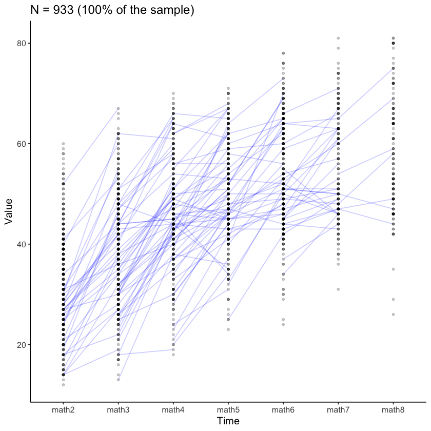
Esaminiamo le traiettorie di crescita nel campione per la matematica.
plot_trajectories(
    data = nlsy_multi_data,
    id_var = "id",
    var_list = x_var_list,
    xlab = "Time", ylab = "Value",
    connect_missing = FALSE,
    # random_sample_frac = 0.018,
    title_n = TRUE
)
Warning message:
“Removed 2787 rows containing missing values or values outside the scale range (`geom_line()`).”
Warning message:
“Removed 4310 rows containing missing values or values outside the scale range (`geom_point()`).”
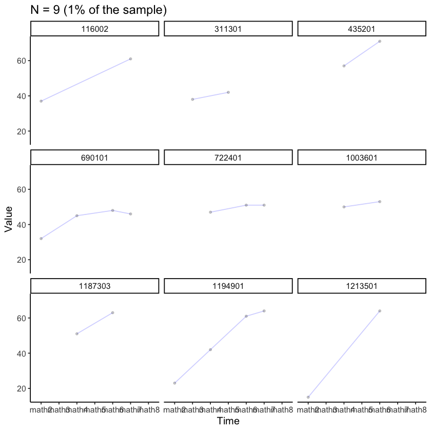
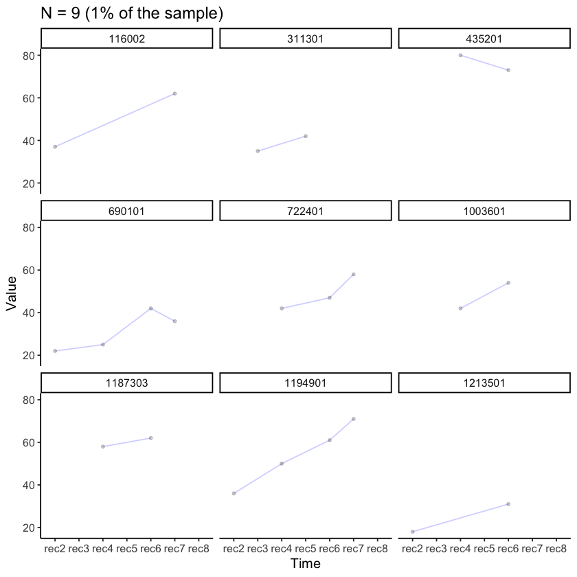
Esaminiamo i dati di alcuni soggetti presi a caso.
plot_trajectories(
    data = nlsy_multi_data,
    id_var = "id",
    var_list = x_var_list,
    xlab = "Time", ylab = "Value",
    connect_missing = TRUE,
    random_sample_frac = 0.01,
    title_n = TRUE) +
  facet_wrap(~id)
Warning message:
“Removed 40 rows containing missing values or values outside the scale range (`geom_point()`).”
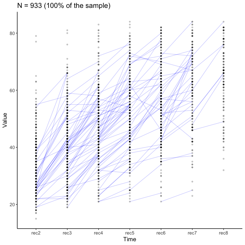
Esaminiamo le curve di crescita per la comprensione nella lettura.
plot_trajectories(
    data = nlsy_multi_data,
    id_var = "id",
    var_list = y_var_list,
    xlab = "Time", ylab = "Value",
    connect_missing = FALSE,
    # random_sample_frac = 0.018,
    title_n = TRUE
)
Warning message:
“Removed 2804 rows containing missing values or values outside the scale range (`geom_line()`).”
Warning message:
“Removed 4317 rows containing missing values or values outside the scale range (`geom_point()`).”
plot_trajectories(
    data = nlsy_multi_data,
    id_var = "id",
    var_list = y_var_list,
    xlab = "Time", ylab = "Value",
    connect_missing = TRUE,
    random_sample_frac = 0.01,
    title_n = TRUE) +
  facet_wrap(~id)
Warning message:
“Removed 40 rows containing missing values or values outside the scale range (`geom_point()`).”
Adattiamo ora quattro modelli di complessità crescente. Il primo modello ipotizza che i parametri di accoppiamento da matematica a lettura e da lettura a matematica siano pari a zero. È il modello baseline. Il secondo modello ipotizza un effetto da lettura a matematica. Il terzo modello ipotizza un effetto da matematica a lettura. Il quarto modello ipotizza la presenza di entrambi i parametri di accoppiamento.
# baseline: no coupling
multi1_lavaan_results <- fit_bi_lcsm(
    data = nlsy_multi_data,
    var_x = x_var_list,
    var_y = y_var_list,
    model_x = list(alpha_constant = TRUE, beta = TRUE, phi = TRUE),
    model_y = list(alpha_constant = TRUE, beta = TRUE, phi = TRUE),
    coupling = list(xi_lag_xy = FALSE, xi_lag_yx = FALSE)
)

# reading affects change in math
multi2_lavaan_results <- fit_bi_lcsm(
    data = nlsy_multi_data,
    var_x = x_var_list,
    var_y = y_var_list,
    model_x = list(alpha_constant = TRUE, beta = TRUE, phi = TRUE),
    model_y = list(alpha_constant = TRUE, beta = TRUE, phi = TRUE),
    coupling = list(xi_lag_xy = TRUE, xi_lag_yx = FALSE)
)

# math affects change in reading
multi3_lavaan_results <- fit_bi_lcsm(
    data = nlsy_multi_data,
    var_x = x_var_list,
    var_y = y_var_list,
    model_x = list(alpha_constant = TRUE, beta = TRUE, phi = TRUE),
    model_y = list(alpha_constant = TRUE, beta = TRUE, phi = TRUE),
    coupling = list(xi_lag_xy = FALSE, xi_lag_yx = TRUE)
)

# both
multi4_lavaan_results <- fit_bi_lcsm(
    data = nlsy_multi_data,
    var_x = x_var_list,
    var_y = y_var_list,
    model_x = list(alpha_constant = TRUE, beta = TRUE, phi = TRUE),
    model_y = list(alpha_constant = TRUE, beta = TRUE, phi = TRUE),
    coupling = list(xi_lag_xy = TRUE, xi_lag_yx = TRUE)
)
Warning message in lav_data_full(data = data, group = group, cluster = cluster, :
“lavaan WARNING: some cases are empty and will be ignored:
  741”
Warning message in lav_data_full(data = data, group = group, cluster = cluster, :
“lavaan WARNING:
    due to missing values, some pairwise combinations have less than
    10% coverage; use lavInspect(fit, "coverage") to investigate.”
Warning message in lav_mvnorm_missing_h1_estimate_moments(Y = X[[g]], wt = WT[[g]], :
“lavaan WARNING:
    Maximum number of iterations reached when computing the sample
    moments using EM; use the em.h1.iter.max= argument to increase the
    number of iterations”
Warning message in lav_data_full(data = data, group = group, cluster = cluster, :
“lavaan WARNING: some cases are empty and will be ignored:
  741”
Warning message in lav_data_full(data = data, group = group, cluster = cluster, :
“lavaan WARNING:
    due to missing values, some pairwise combinations have less than
    10% coverage; use lavInspect(fit, "coverage") to investigate.”
Warning message in lav_mvnorm_missing_h1_estimate_moments(Y = X[[g]], wt = WT[[g]], :
“lavaan WARNING:
    Maximum number of iterations reached when computing the sample
    moments using EM; use the em.h1.iter.max= argument to increase the
    number of iterations”
È ora possibile fare un confronto tra i vari modelli. Di seguito riportiamo la statistica BIC (valori minori sono preferibili). Dalle statistiche BIC emerge che il modello baseline è da preferire.
c(
    extract_fit(multi1_lavaan_results)$bic,
    extract_fit(multi2_lavaan_results)$bic,
    extract_fit(multi3_lavaan_results)$bic,
    extract_fit(multi4_lavaan_results)$bic
) |> print()
[1] 31518.91 31524.44 31526.38 31521.89
Eseguiamo ora i test del rapporto tra verosimiglianze tra i vari modelli.
lavTestLRT(multi1_lavaan_results, multi2_lavaan_results) |>
    print()
Scaled Chi-Squared Difference Test (method = "satorra.bentler.2001")

lavaan NOTE:
    The "Chisq" column contains standard test statistics, not the
    robust test that should be reported per model. A robust difference
    test is a function of two standard (not robust) statistics.

                      Df   AIC   BIC  Chisq Chisq diff Df diff Pr(>Chisq)
multi2_lavaan_results 97 31418 31524 179.14
multi1_lavaan_results 98 31417 31519 180.46     3.4354       1    0.06381 .
---
Signif. codes:  0 '***' 0.001 '**' 0.01 '*' 0.05 '.' 0.1 ' ' 1
lavTestLRT(multi1_lavaan_results, multi3_lavaan_results) |>
    print()
Warning message in lavTestLRT(multi1_lavaan_results, multi3_lavaan_results):
"lavaan WARNING:
    Some restricted models fit better than less restricted models;
    either these models are not nested, or the less restricted model
    failed to reach a global optimum. Smallest difference =
    -0.633896069371474"
Scaled Chi-Squared Difference Test (method = "satorra.bentler.2001")

lavaan NOTE:
    The "Chisq" column contains standard test statistics, not the
    robust test that should be reported per model. A robust difference
    test is a function of two standard (not robust) statistics.

                      Df   AIC   BIC  Chisq Chisq diff Df diff Pr(>Chisq)
multi3_lavaan_results 97 31420 31526 181.09
multi1_lavaan_results 98 31417 31519 180.46   -0.17583       1          1
lavTestLRT(multi1_lavaan_results, multi4_lavaan_results) |>
    print()
Scaled Chi-Squared Difference Test (method = "satorra.bentler.2001")

lavaan NOTE:
    The "Chisq" column contains standard test statistics, not the
    robust test that should be reported per model. A robust difference
    test is a function of two standard (not robust) statistics.

                      Df   AIC   BIC  Chisq Chisq diff Df diff Pr(>Chisq)
multi4_lavaan_results 96 31411 31522 169.76
multi1_lavaan_results 98 31417 31519 180.46     5.9923       2    0.04998 *
---
Signif. codes:  0 '***' 0.001 '**' 0.01 '*' 0.05 '.' 0.1 ' ' 1
Anche in questo caso non vi è evidenza che la presenza dei fattori di accoppiamento migliori l’adattamento del modello ai dati.
Per motivi didattici, però, proseguiamo l’analisi ipotizzando una presenza di entrambe le classi di parametri di accoppiamento (da comprensione nella lettura a matematica e viceversa).
multi4_lavaan_syntax <- fit_bi_lcsm(
    data = nlsy_multi_data,
    var_x = x_var_list,
    var_y = y_var_list,
    model_x = list(alpha_constant = TRUE, beta = TRUE, phi = TRUE),
    model_y = list(alpha_constant = TRUE, beta = TRUE, phi = TRUE),
    coupling = list(xi_lag_xy = TRUE, xi_lag_yx = TRUE),
    return_lavaan_syntax = TRUE
)
Di seguito riportiamo il path diagram del modello prescelto.
# Plot the results
plot_lcsm(
    lavaan_object = multi4_lavaan_results,
    lavaan_syntax = multi4_lavaan_syntax,
    edge.label.cex = .9,
    lcsm_colours = TRUE,
    lcsm = "bivariate"
)
Esaminiamo la bontà di adattamento.
extract_fit(multi4_lavaan_results) |> print()
# A tibble: 1 x 8
  model chisq  npar    aic    bic   cfi  rmsea  srmr
  <chr> <dbl> <dbl>  <dbl>  <dbl> <dbl>  <dbl> <dbl>
1 1      170.    23 31411. 31522. 0.972 0.0287 0.108
Notiamo che le informazioni sull’adattamento del modello fornite da lcsm indicano che il modello di cambiamento duale si adatta bene ai dati con forti indici di adattamento globale (ad esempio, RMSEA inferiore a 0.05, CFI > 0.95).
Esaminiamo i parametri.
extract_param(multi4_lavaan_results) |> print()
# A tibble: 23 x 8
   label       estimate std.error statistic  p.value   std.lv  std.all  std.nox
   <chr>          <dbl>     <dbl>     <dbl>    <dbl>    <dbl>    <dbl>    <dbl>
 1 gamma_lx1   32.5        0.543    60.0    0         4.08     4.08     4.08
 2 sigma2_lx1  63.8        4.90     13.0    0         1        1        1
 3 sigma2_ux   29.6        1.71     17.3    0        29.6      0.317    0.317
 4 alpha_g2     7.82       2.18      3.58   0.000338  2.37     2.37     2.37
 5 sigma2_g2   10.9        8.19      1.33   0.183     1        1        1
 6 sigma_g2lx1  0.216      6.81      0.0317 0.975     0.00819  0.00819  0.00819
 7 beta_x      -0.00771    0.0563   -0.137  0.891    -0.0186  -0.0186  -0.0186
 8 phi_x        4.73       3.30      1.43   0.152     3.89     3.89     3.89
 9 gamma_ly1   33.8        0.422    80.1    0         3.53     3.53     3.53
10 sigma2_ly1  91.5        9.02     10.1    0         1        1        1
# i 13 more rows
L’output completo è fornito qui di seguito.
out = summary(multi4_lavaan_results)
print(out)
lavaan 0.6.17 ended normally after 484 iterations

  Estimator                                         ML
  Optimization method                           NLMINB
  Number of model parameters                        67
  Number of equality constraints                    44

                                                  Used       Total
  Number of observations                           932         933
  Number of missing patterns                        66

Model Test User Model:
                                              Standard      Scaled
  Test Statistic                               169.764     182.983
  Degrees of freedom                                96          96
  P-value (Chi-square)                           0.000       0.000
  Scaling correction factor                                  0.928
    Yuan-Bentler correction (Mplus variant)

Parameter Estimates:

  Standard errors                             Sandwich
  Information bread                           Observed
  Observed information based on                Hessian

Latent Variables:
                   Estimate  Std.Err  z-value  P(>|z|)
  lx1 =~
    x1                1.000
  lx2 =~
    x2                1.000
  lx3 =~
    x3                1.000
  lx4 =~
    x4                1.000
  lx5 =~
    x5                1.000
  lx6 =~
    x6                1.000
  lx7 =~
    x7                1.000
  dx2 =~
    lx2               1.000
  dx3 =~
    lx3               1.000
  dx4 =~
    lx4               1.000
  dx5 =~
    lx5               1.000
  dx6 =~
    lx6               1.000
  dx7 =~
    lx7               1.000
  g2 =~
    dx2               1.000
    dx3               1.000
    dx4               1.000
    dx5               1.000
    dx6               1.000
    dx7               1.000
  ly1 =~
    y1                1.000
  ly2 =~
    y2                1.000
  ly3 =~
    y3                1.000
  ly4 =~
    y4                1.000
  ly5 =~
    y5                1.000
  ly6 =~
    y6                1.000
  ly7 =~
    y7                1.000
  dy2 =~
    ly2               1.000
  dy3 =~
    ly3               1.000
  dy4 =~
    ly4               1.000
  dy5 =~
    ly5               1.000
  dy6 =~
    ly6               1.000
  dy7 =~
    ly7               1.000
  j2 =~
    dy2               1.000
    dy3               1.000
    dy4               1.000
    dy5               1.000
    dy6               1.000
    dy7               1.000

Regressions:
                   Estimate  Std.Err  z-value  P(>|z|)
  lx2 ~
    lx1               1.000
  lx3 ~
    lx2               1.000
  lx4 ~
    lx3               1.000
  lx5 ~
    lx4               1.000
  lx6 ~
    lx5               1.000
  lx7 ~
    lx6               1.000
  dx2 ~
    lx1     (bt_x)   -0.008    0.056   -0.137    0.891
  dx3 ~
    lx2     (bt_x)   -0.008    0.056   -0.137    0.891
  dx4 ~
    lx3     (bt_x)   -0.008    0.056   -0.137    0.891
  dx5 ~
    lx4     (bt_x)   -0.008    0.056   -0.137    0.891
  dx6 ~
    lx5     (bt_x)   -0.008    0.056   -0.137    0.891
  dx7 ~
    lx6     (bt_x)   -0.008    0.056   -0.137    0.891
  dx3 ~
    dx2     (ph_x)    4.731    3.304    1.432    0.152
  dx4 ~
    dx3     (ph_x)    4.731    3.304    1.432    0.152
  dx5 ~
    dx4     (ph_x)    4.731    3.304    1.432    0.152
  dx6 ~
    dx5     (ph_x)    4.731    3.304    1.432    0.152
  dx7 ~
    dx6     (ph_x)    4.731    3.304    1.432    0.152
  ly2 ~
    ly1               1.000
  ly3 ~
    ly2               1.000
  ly4 ~
    ly3               1.000
  ly5 ~
    ly4               1.000
  ly6 ~
    ly5               1.000
  ly7 ~
    ly6               1.000
  dy2 ~
    ly1     (bt_y)    0.076    0.041    1.832    0.067
  dy3 ~
    ly2     (bt_y)    0.076    0.041    1.832    0.067
  dy4 ~
    ly3     (bt_y)    0.076    0.041    1.832    0.067
  dy5 ~
    ly4     (bt_y)    0.076    0.041    1.832    0.067
  dy6 ~
    ly5     (bt_y)    0.076    0.041    1.832    0.067
  dy7 ~
    ly6     (bt_y)    0.076    0.041    1.832    0.067
  dy3 ~
    dy2     (ph_y)   -5.985    3.231   -1.852    0.064
  dy4 ~
    dy3     (ph_y)   -5.985    3.231   -1.852    0.064
  dy5 ~
    dy4     (ph_y)   -5.985    3.231   -1.852    0.064
  dy6 ~
    dy5     (ph_y)   -5.985    3.231   -1.852    0.064
  dy7 ~
    dy6     (ph_y)   -5.985    3.231   -1.852    0.064
  dx3 ~
    dy2   (x_lg_x)   -4.864    2.915   -1.668    0.095
  dx4 ~
    dy3   (x_lg_x)   -4.864    2.915   -1.668    0.095
  dx5 ~
    dy4   (x_lg_x)   -4.864    2.915   -1.668    0.095
  dx6 ~
    dy5   (x_lg_x)   -4.864    2.915   -1.668    0.095
  dx7 ~
    dy6   (x_lg_x)   -4.864    2.915   -1.668    0.095
  dy3 ~
    dx2   (x_lg_y)    5.830    3.721    1.566    0.117
  dy4 ~
    dx3   (x_lg_y)    5.830    3.721    1.566    0.117
  dy5 ~
    dx4   (x_lg_y)    5.830    3.721    1.566    0.117
  dy6 ~
    dx5   (x_lg_y)    5.830    3.721    1.566    0.117
  dy7 ~
    dx6   (x_lg_y)    5.830    3.721    1.566    0.117

Covariances:
                   Estimate  Std.Err  z-value  P(>|z|)
  lx1 ~~
    g2 (sgm_g2lx1)    0.216    6.811    0.032    0.975
  ly1 ~~
    j2 (sgm_j2ly1)   -4.945    7.807   -0.633    0.526
 .x1 ~~
   .y1      (sgm_)    3.888    1.514    2.568    0.010
 .x2 ~~
   .y2      (sgm_)    3.888    1.514    2.568    0.010
 .x3 ~~
   .y3      (sgm_)    3.888    1.514    2.568    0.010
 .x4 ~~
   .y4      (sgm_)    3.888    1.514    2.568    0.010
 .x5 ~~
   .y5      (sgm_)    3.888    1.514    2.568    0.010
 .x6 ~~
   .y6      (sgm_)    3.888    1.514    2.568    0.010
 .x7 ~~
   .y7      (sgm_)    3.888    1.514    2.568    0.010
  lx1 ~~
    l1      (s_11)   52.706    5.478    9.622    0.000
  g2 ~~
    l1 (sgm_g2ly1)    2.305    6.817    0.338    0.735
  lx1 ~~
    j2 (sgm_j2lx1)   -4.187    6.344   -0.660    0.509
  g2 ~~
    j2      (s_22)   14.752   10.409    1.417    0.156

Intercepts:
                   Estimate  Std.Err  z-value  P(>|z|)
    lx1  (gmm_lx1)   32.540    0.543   59.963    0.000
   .lx2               0.000
   .lx3               0.000
   .lx4               0.000
   .lx5               0.000
   .lx6               0.000
   .lx7               0.000
   .x1                0.000
   .x2                0.000
   .x3                0.000
   .x4                0.000
   .x5                0.000
   .x6                0.000
   .x7                0.000
   .dx2               0.000
   .dx3               0.000
   .dx4               0.000
   .dx5               0.000
   .dx6               0.000
   .dx7               0.000
    g2   (alph_g2)    7.822    2.182    3.584    0.000
    ly1  (gmm_ly1)   33.762    0.422   80.067    0.000
   .ly2               0.000
   .ly3               0.000
   .ly4               0.000
   .ly5               0.000
   .ly6               0.000
   .ly7               0.000
   .y1                0.000
   .y2                0.000
   .y3                0.000
   .y4                0.000
   .y5                0.000
   .y6                0.000
   .y7                0.000
   .dy2               0.000
   .dy3               0.000
   .dy4               0.000
   .dy5               0.000
   .dy6               0.000
   .dy7               0.000
    j2   (alph_j2)    5.289    1.598    3.310    0.001

Variances:
                   Estimate  Std.Err  z-value  P(>|z|)
    lx1 (sgm2_lx1)   63.761    4.904   13.001    0.000
   .lx2               0.000
   .lx3               0.000
   .lx4               0.000
   .lx5               0.000
   .lx6               0.000
   .lx7               0.000
   .x1    (sgm2_x)   29.553    1.713   17.251    0.000
   .x2    (sgm2_x)   29.553    1.713   17.251    0.000
   .x3    (sgm2_x)   29.553    1.713   17.251    0.000
   .x4    (sgm2_x)   29.553    1.713   17.251    0.000
   .x5    (sgm2_x)   29.553    1.713   17.251    0.000
   .x6    (sgm2_x)   29.553    1.713   17.251    0.000
   .x7    (sgm2_x)   29.553    1.713   17.251    0.000
   .dx2               0.000
   .dx3               0.000
   .dx4               0.000
   .dx5               0.000
   .dx6               0.000
   .dx7               0.000
    g2   (sgm2_g2)   10.913    8.188    1.333    0.183
    ly1 (sgm2_ly1)   91.477    9.025   10.136    0.000
   .ly2               0.000
   .ly3               0.000
   .ly4               0.000
   .ly5               0.000
   .ly6               0.000
   .ly7               0.000
   .y1    (sgm2_y)   30.320    1.940   15.632    0.000
   .y2    (sgm2_y)   30.320    1.940   15.632    0.000
   .y3    (sgm2_y)   30.320    1.940   15.632    0.000
   .y4    (sgm2_y)   30.320    1.940   15.632    0.000
   .y5    (sgm2_y)   30.320    1.940   15.632    0.000
   .y6    (sgm2_y)   30.320    1.940   15.632    0.000
   .y7    (sgm2_y)   30.320    1.940   15.632    0.000
   .dy2               0.000
   .dy3               0.000
   .dy4               0.000
   .dy5               0.000
   .dy6               0.000
   .dy7               0.000
    j2   (sgm2_j2)   20.928   12.318    1.699    0.089
85.1.1. Interpretazione#
Le stime dei parametri di questo modello descrivono le traiettorie medie e individuali per la matematica e la comprensione della lettura, nonché le loro associazioni nel tempo. Le traiettorie medie per la matematica e la comprensione della lettura iniziano rispettivamente a 32.27 e 33.99. Da lì, le traiettorie medie sono descritte dalle rispettive equazioni di cambiamento.
Per l’equazione di cambiamento della matematica, la media della componente di cambiamento costante è 15.82 e indica l’aumento costante ogni anno. La media della componente di cambiamento proporzionale è -0.27, il che indica un effetto limitativo (il coefficiente è negativo) sul cambiamento in matematica dovuto ai punteggi precedenti di matematica. Il modello assume l’assenza di un effetto di accoppiamento (0).
Per l’equazione di cambiamento della comprensione nella lettura, la media della componente di cambiamento costante è 12.59 e indica l’aumento costante ogni anno. La media della componente di cambiamento proporzionale è -0.15, il che indica un effetto limitativo (il coefficiente è negativo) sul cambiamento nella comprensione nella lettura dovuto ai punteggi precedenti di comprensione nella lettura. Il modello assume l’assenza di un effetto di accoppiamento (0).
Poniamoci ora il problema di creare una figura che riporta le traiettorie individuali previste dal modello bivariato. Per creare la figura dobbiamo innanzitutto recuperare la sintassi lavaan del modello duale.
Otteniamo i punteggi fattoriali.
nlsy_predicted <- cbind(
    nlsy_multi_data$id,
    as.data.frame(lavPredict(multi4_lavaan_results, type = "yhat"))
)
names(nlsy_predicted)[1] <- "id"
#looking at data
head(nlsy_predicted)
| id | x1 | x2 | x3 | x4 | x5 | x6 | x7 | y1 | y2 | y3 | y4 | y5 | y6 | y7 | |
|---|---|---|---|---|---|---|---|---|---|---|---|---|---|---|---|
| <int> | <dbl> | <dbl> | <dbl> | <dbl> | <dbl> | <dbl> | <dbl> | <dbl> | <dbl> | <dbl> | <dbl> | <dbl> | <dbl> | <dbl> | |
| 1 | 201 | 33.15176 | 40.43844 | 46.60271 | 50.77319 | 54.73281 | 57.07988 | 59.47240 | 31.45715 | 38.76294 | 45.37727 | 50.08929 | 54.92148 | 58.17234 | 61.73385 |
| 2 | 303 | 24.39926 | 28.98397 | 35.86019 | 37.92657 | 42.93685 | 43.62843 | 47.28636 | 24.58506 | 28.56551 | 35.75247 | 37.65318 | 43.29687 | 44.12950 | 48.64298 |
| 3 | 2702 | 47.54951 | 53.80030 | 60.98284 | 64.20800 | 69.19670 | 70.71387 | 74.12672 | 37.03671 | 42.91439 | 50.50044 | 53.87010 | 59.66067 | 61.68289 | 66.17441 |
| 4 | 4303 | 37.47188 | 42.91769 | 50.78769 | 53.29757 | 58.99872 | 59.89817 | 64.02936 | 31.37796 | 36.16723 | 44.40361 | 46.76698 | 53.21213 | 54.32159 | 59.45710 |
| 5 | 5002 | 33.15122 | 42.56383 | 47.98136 | 53.84208 | 56.81824 | 60.51675 | 61.77965 | 37.95614 | 47.91670 | 53.89218 | 60.88241 | 64.91407 | 70.14310 | 72.81414 |
| 6 | 5005 | 36.26630 | 45.51709 | 49.89202 | 55.82861 | 57.95578 | 61.83941 | 62.39880 | 47.08275 | 57.06728 | 61.98182 | 69.18891 | 72.32670 | 77.84997 | 79.75528 |
Convertiamo i dati in formato long.
predicted_long <- reshape(
       data = nlsy_predicted,
       varying = c(
              "x1", "x2", "x3", "x4", "x5", "x6", "x7",
              "y1", "y2", "y3", "y4", "y5", "y6", "y7"
       ),
       timevar = c("grade"),
       idvar = c("id"),
       direction = "long", sep = ""
)

#sorting for easy viewing
#reorder by id and day
predicted_long <- predicted_long[order(predicted_long$id,predicted_long$grade), ]

#looking at the long data
head(predicted_long, 14)
| id | grade | x | y | |
|---|---|---|---|---|
| <int> | <dbl> | <dbl> | <dbl> | |
| 201.1 | 201 | 1 | 33.15176 | 31.45715 |
| 201.2 | 201 | 2 | 40.43844 | 38.76294 |
| 201.3 | 201 | 3 | 46.60271 | 45.37727 |
| 201.4 | 201 | 4 | 50.77319 | 50.08929 |
| 201.5 | 201 | 5 | 54.73281 | 54.92148 |
| 201.6 | 201 | 6 | 57.07988 | 58.17234 |
| 201.7 | 201 | 7 | 59.47240 | 61.73385 |
| 303.1 | 303 | 1 | 24.39926 | 24.58506 |
| 303.2 | 303 | 2 | 28.98397 | 28.56551 |
| 303.3 | 303 | 3 | 35.86019 | 35.75247 |
| 303.4 | 303 | 4 | 37.92657 | 37.65318 |
| 303.5 | 303 | 5 | 42.93685 | 43.29687 |
| 303.6 | 303 | 6 | 43.62843 | 44.12950 |
| 303.7 | 303 | 7 | 47.28636 | 48.64298 |
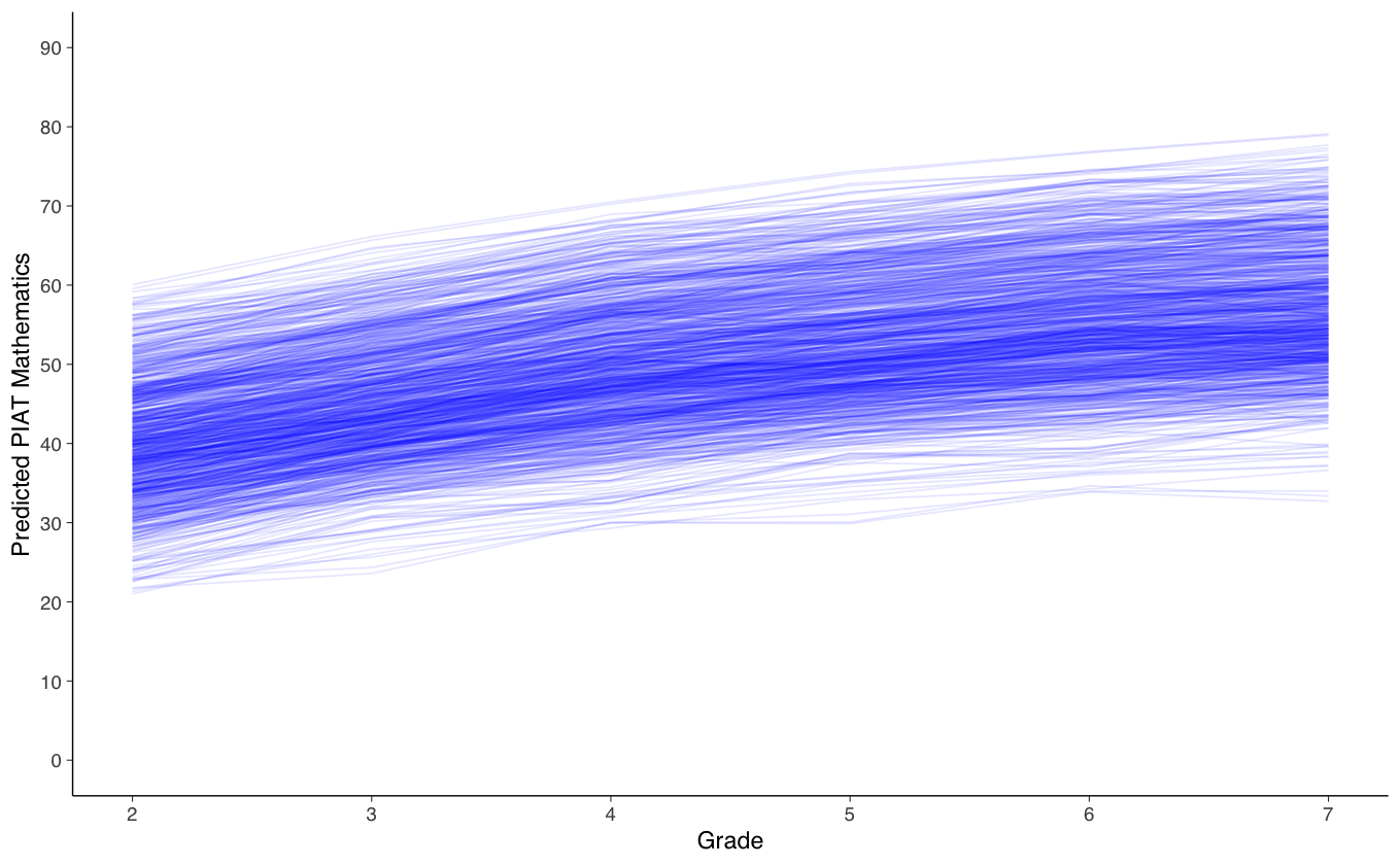
Creiamo un grafico del cambiamento intra-individuale per la matematica.
ggplot(data = predicted_long, aes(x = grade, y = x, group = id)) +
  #geom_point(color="blue") +
  geom_line(color="blue", alpha= 0.1) +
  xlab("Grade") +
  ylab("Predicted PIAT Mathematics") +
  scale_x_continuous(limits=c(2,7), breaks=seq(2,8,by=1)) +
  scale_y_continuous(limits=c(0,90), breaks=seq(0,90,by=10))
Warning message:
"Removed 939 rows containing missing values (`geom_line()`)."
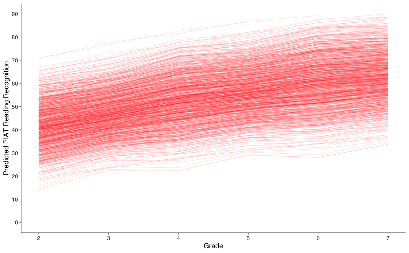
Creiamo un grafico del cambiamento intra-individuale per la comprensione nella lettura.
ggplot(data = predicted_long, aes(x = grade, y = y, group = id)) +
  #geom_point(color="red") +
  geom_line(color="red", alpha= 0.1) +
  xlab("Grade") +
  ylab("Predicted PIAT Reading Recognition") +
  scale_x_continuous(limits=c(2,7), breaks=seq(2,8,by=1)) +
  scale_y_continuous(limits=c(0,90), breaks=seq(0,90,by=10))
Warning message:
"Removed 942 rows containing missing values (`geom_line()`)."
Esaminiamo gli effetti combinati dei cambiamenti nelle due variabili.
# reshaping wide to long
data_long <- reshape(
       data = nlsy_multi_data,
       varying = c(
              "math2", "math3", "math4", "math5", "math6", "math7", "math8",
              "rec2", "rec3", "rec4", "rec5", "rec6", "rec7", "rec8"
       ),
       timevar = c("grade"),
       idvar = c("id"),
       direction = "long", sep = ""
)

#sorting for easy viewing
#reorder by id and day
data_long <- data_long[order(data_long$id,data_long$grade), ]

#looking at the long data
head(data_long, 8)
| id | grade | math | rec | |
|---|---|---|---|---|
| <int> | <dbl> | <int> | <int> | |
| 201.2 | 201 | 2 | NA | NA |
| 201.3 | 201 | 3 | 38 | 35 |
| 201.4 | 201 | 4 | NA | NA |
| 201.5 | 201 | 5 | 55 | 52 |
| 201.6 | 201 | 6 | NA | NA |
| 201.7 | 201 | 7 | NA | NA |
| 201.8 | 201 | 8 | NA | NA |
| 303.2 | 303 | 2 | 26 | 26 |
#creating a grid of starting values
df <- expand.grid(math=seq(10, 90, 5), rec=seq(10, 90, 5))

#calculating change scores for each starting value
#changes in math based on output from model
df$dm <- with(df, 15.09 - 0.293*math + 0.053*rec)
#changes in reading based on output from model
df$dr <- with(df, 10.89 - 0.495*rec + 0.391*math)

#Plotting vector field with .25 unit time change
ggplot(data = df, aes(x = x, y = y)) +
  geom_point(data=data_long, aes(x=rec, y=math), alpha=.1) +
  stat_ellipse(data=data_long, aes(x=rec, y=math)) +
  geom_segment(aes(x = rec, y = math, xend = rec+.25*dr, yend = math+.25*dm), arrow = arrow(length = unit(0.1, "cm"))) +
  xlab("Reading Recognition") +
  ylab("Mathematics") +
  scale_x_continuous(limits=c(10,90), breaks=seq(10,90,by=10)) +
  scale_y_continuous(limits=c(10,90), breaks=seq(10,90,by=10))
Warning message:
"Removed 4317 rows containing non-finite values (`stat_ellipse()`)."
Warning message:
"Removed 4317 rows containing missing values (`geom_point()`)."
Warning message:
"Removed 1 rows containing missing values (`geom_segment()`)."
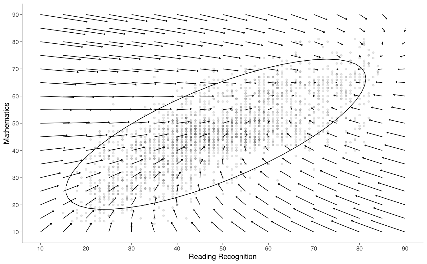
Il grafico rappresenta l’evoluzione delle variabili nel tempo. Le frecce del campo vettoriale indicano le variazioni previste nello spazio bivariato per un intervallo di tempo di 0.25 unità. Si osserva che i dati si concentrano principalmente all’interno dell’ellisse di confidenza al 95%. Al di fuori di questa area, i vettori direzionali sono interpolati sulla base delle osservazioni e dei modelli derivati dai dati effettivi (cioè all’interno dell’ellisse). Pertanto, è importante evitare di sovrainterpretare le dinamiche al di fuori dell’ellisse.
La regione dello spazio vettoriale in cui i vettori tendono a zero indica le combinazioni di valori delle due variabili per cui non si prevedono ulteriori cambiamenti. L’aspetto più interessante del grafico non è tanto il risultato finale del processo, quanto la descrizione della forza e della direzione del cambiamento per ogni combinazione di valori delle due variabili considerate.