36. Invarianza di misurazione#
In questo capitolo, esaminiamo come il modello a fattore comune possa essere utilizzato per studiare i cambiamenti nei fattori comuni attraverso l’uso di modelli di crescita latente. Ci concentriamo sui fattori comuni misurati da variabili osservate con punteggio continuo.
Un concetto chiave è stabilire una metrica comune per le variabili latenti nel tempo. A differenza delle variabili osservate, le variabili latenti non hanno una scala intrinseca e longitudinalmente è necessario che quella scala sia la stessa nel tempo. Questo viene fatto testando l’invarianza fattoriale.
In questo tutorial, introduciamo il test di invarianza di misura nel contesto di un modello a fattore longitudinale e come un modello di crescita latente di secondo ordine possa essere utilizzato per descrivere il cambiamento in un fattore latente. Questo tutorial segue l’esempio fornito nel Capitolo 14 Grimm et al. [GRE16]. Utilizzando dati con tre misurazioni temporali succesive dall’ECLS-K, testiamo l’invarianza fattoriale e quindi utilizziamo un modello di crescita di secondo ordine per descrivere il cambiamento nei punteggi del fattore nel tempo.
36.1. Invarianza fattoriale longitudinale#
L’invarianza fattoriale longitudinale si riferisce all’equivalenza di alcuni parametri del modello a fattore comune nel tempo. Avere una struttura fattoriale invariante è importante per l’utilizzo dell’analisi fattoriale come strumento di indagine scientifica. I fattori non hanno un’unità di misura o un significato intrinseco e la loro interpretazione deriva dalle loro relazioni con le variabili osservate. Se un fattore deve essere trattato come lo stesso in diverse occasioni temporali di misurazione, l’associazione di quel fattore con altre variabili deve rimanere costante nel tempo.
Il test di invarianza fattoriale è una procedura multi-step che comporta l’adattamento di quattro modelli con un numero crescente di vincoli: il modello di invarianza configurale, il modello di invarianza debole, il modello di invarianza forte e il modello di invarianza rigorosa.
Il modello di invarianza configurale richiede che il numero di fattori e la struttura delle saturazioni fattoriali siano uguali nelle diverse occasioni di misurazione. Altre caratteristiche come le varianze e le medie dei fattori possono variare. I fattori estratti in ogni occasione possono essere interpretati in modo simile, ma non possono essere considerati come misure di costrutti identici o sulla stessa scala.
I modelli di invarianza configurale sono usati come punto di partenza per confrontare altri modelli con vincoli maggiori. Questi modelli presuppongono che lo stesso numero di fattori sia presente in ogni occasione di misurazione, ma questa ipotesi potrebbe non essere vera. I ricercatori dovrebbero verificare che le ipotesi dell’invarianza configurale siano soddisfatte prima di procedere con i successivi test di invarianza.
L’invarianza fattoriale debole è il modello meno vincolato tra i tre modelli di invarianza metrica descritti da Meredith (1993). Questo modello richiede che la matrice delle saturazioni fattoriali sia uguale in tutte le rilevazioni temporali, ma non impone altre restrizioni. Poiché la matrice delle saturazioni fattoriali definisce le covarianze tra le variabili osservate, l’invarianza fattoriale debole crea strutture di covarianza proporzionali nel tempo.
L’invarianza forte fornisce un livello più elevato di invarianza di misura vincolando le intercette delle variabili osservate ad essere uguali nelle diverse occasioni di misurazione e consentendo al contempo al vettore delle medie delle variabili latenti di variare nel tempo. Ciò significa che tutti i cambiamenti longitudinali nelle medie delle variabili osservate sono spiegati dal fattore(i) comune(i).
L’invarianza fattoriale rigorosa è il modello di fattore longitudinale con i vincoli più forti. Oltre ai vincoli sulle saturazioni fattoriali e sulle intercette delle variabili osservate, questo modello richiede che le varianze uniche siano uguali nelle diverse occasioni di misurazione. In questo modello, tutti i cambiamenti longitudinali nelle medie osservate, nelle varianze e nelle covarianze sono attribuiti ai cambiamenti nei fattori comuni nel tempo.
36.2. Un esempio concreto#
Questo tutorial segue l’esempio del Capitolo 14 di Grimm et al. [GRE16]. Utilizzando dati relativi a 3 misurazioni dell’ECLS-K, testiamo l’invarianza fattoriale e poi usiamo un modello di crescita latente di secondo ordine per descrivere il cambiamento nei punteggi fattoriali nel tempo.
Carichiamo i pacchetti necessari.
Leggiamo i dati.
filepath <- "https://raw.githubusercontent.com/LRI-2/Data/main/GrowthModeling/ECLS_Science.dat"
# read in the text data file using the url() function
dat <- read.table(file = url(filepath), na.strings = ".")

names(dat) <- c(
  "id", "s_g3", "r_g3", "m_g3", "s_g5", "r_g5", "m_g5", "s_g8",
  "r_g8", "m_g8", "st_g3", "rt_g3", "mt_g3", "st_g5", "rt_g5",
  "mt_g5", "st_g8", "rt_g8", "mt_g8"
)

# selecting only the variables of interest
dat <- dat[, c(
  "id", "s_g3", "r_g3", "m_g3", "s_g5", "r_g5", "m_g5", "s_g8",
  "r_g8", "m_g8"
)]
head(dat, 10)
| id | s_g3 | r_g3 | m_g3 | s_g5 | r_g5 | m_g5 | s_g8 | r_g8 | m_g8 | |
|---|---|---|---|---|---|---|---|---|---|---|
| <dbl> | <dbl> | <dbl> | <dbl> | <dbl> | <dbl> | <dbl> | <dbl> | <dbl> | <dbl> | |
| 1 | 1 | NA | NA | NA | NA | NA | NA | NA | NA | NA |
| 2 | 3 | NA | NA | NA | NA | NA | NA | NA | NA | NA |
| 3 | 8 | NA | NA | NA | NA | NA | NA | 103.90 | 204.10 | 166.67 |
| 4 | 16 | 51.57 | 142.18 | 115.59 | 65.94 | 141.02 | 133.67 | 86.90 | 169.83 | 156.67 |
| 5 | 28 | NA | NA | NA | NA | NA | NA | NA | NA | NA |
| 6 | 44 | NA | NA | NA | NA | NA | NA | NA | NA | NA |
| 7 | 46 | 72.09 | 154.43 | 96.87 | 79.44 | 170.57 | 116.28 | 89.08 | 192.07 | 132.40 |
| 8 | 62 | 34.71 | 106.40 | 87.86 | 47.44 | 145.72 | 104.68 | NA | NA | NA |
| 9 | 66 | NA | NA | NA | NA | NA | NA | NA | NA | NA |
| 10 | 74 | 62.94 | 126.06 | 92.47 | 73.70 | 145.17 | 124.73 | 92.67 | 193.43 | 133.93 |
Otteniamo le statistiche descrittive.
psych::describe(dat[, -1]) |>
    print()
     vars    n   mean    sd median trimmed   mad   min    max  range  skew
s_g3    1 1442  50.99 15.62  50.94   50.82 16.76 18.37  92.66  74.29  0.08
r_g3    2 1430 127.66 29.22 126.97  128.44 31.33 51.46 195.82 144.36 -0.21
m_g3    3 1442  99.72 25.54 102.60   99.99 27.71 35.72 159.40 123.68 -0.10
s_g5    4 1135  65.25 16.18  67.53   65.99 16.52 22.57 103.23  80.66 -0.39
r_g5    5 1133 151.09 27.31 152.33  153.10 26.73 64.69 202.22 137.53 -0.62
m_g5    6 1136 124.35 25.17 128.64  126.08 25.14 50.87 169.53 118.66 -0.58
s_g8    7  947  84.89 16.71  88.93   86.88 14.81 29.61 107.90  78.29 -0.99
r_g8    8  941 172.05 27.73 179.70  175.54 24.91 89.15 208.44 119.29 -0.98
m_g8    9  945 142.47 22.50 147.36  145.07 21.23 67.75 172.20 104.45 -0.94
     kurtosis   se
s_g3    -0.59 0.41
r_g3    -0.50 0.77
m_g3    -0.70 0.67
s_g5    -0.49 0.48
r_g5    -0.04 0.81
m_g5    -0.24 0.75
s_g8     0.48 0.54
r_g8     0.24 0.90
m_g8     0.36 0.73
Calcoliamo le correlazioni.
round(cor(dat[, -1], use = "pairwise.complete"), 2) |>
    print()
     s_g3 r_g3 m_g3 s_g5 r_g5 m_g5 s_g8 r_g8 m_g8
s_g3 1.00 0.76 0.71 0.85 0.73 0.68 0.75 0.68 0.66
r_g3 0.76 1.00 0.75 0.73 0.85 0.70 0.70 0.76 0.68
m_g3 0.71 0.75 1.00 0.70 0.72 0.88 0.71 0.66 0.81
s_g5 0.85 0.73 0.70 1.00 0.77 0.74 0.81 0.73 0.70
r_g5 0.73 0.85 0.72 0.77 1.00 0.75 0.74 0.80 0.71
m_g5 0.68 0.70 0.88 0.74 0.75 1.00 0.74 0.68 0.85
s_g8 0.75 0.70 0.71 0.81 0.74 0.74 1.00 0.78 0.78
r_g8 0.68 0.76 0.66 0.73 0.80 0.68 0.78 1.00 0.75
m_g8 0.66 0.68 0.81 0.70 0.71 0.85 0.78 0.75 1.00
corrplot(cor(dat[, -1], use = "pairwise.complete"), order = "original", tl.col = "black", tl.cex = .75)

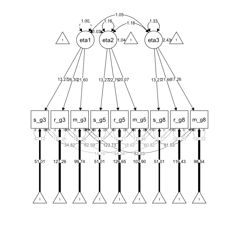
36.2.1. Modello di invarianza configurale#
Il modello di invarianza configurale impone pochi vincoli sulla struttura del fattore nel tempo. L’unico vincolo è che il numero di fattori e la struttura delle saturazioni fattoriali siano uguali nelle diverse occasioni di misurazione. Definiamo un fattore “rendimento accademico” per ciascuna delle 3 occasioni, utilizzando le variabili di matematica, scienze e lettura relative a quella misurazione temporale.
Anche se il fattore comune può essere interpretato in modo simile in ciascuna occasione di misurazione (ad esempio, chiamato “rendimento accademico”), questo modello non impone o assume che i fattori specifici per il tempo misurino lo stesso costrutto o che siano misurati sulla stessa scala.
Definiamo il modello nella sintassi di lavaan.
configural_invar <- " #opening quote
#factor loadings
  eta1 =~ lambda_S*s_g3+ #for identification
          lambda_R3*r_g3+
          lambda_M3*m_g3
  eta2 =~ lambda_S*s_g5+ #for identification
          lambda_R5*r_g5+
          lambda_M5*m_g5
  eta3 =~ lambda_S*s_g8+ #for identification
          lambda_R8*r_g8+
          lambda_M8*m_g8

#latent variable variances
   eta1~~1*eta1 #for scaling
   eta2~~eta2
   eta3~~eta3

#latent variable covariances
   eta1~~eta2
   eta1~~eta3
   eta2~~eta3

#unique variances
   s_g3~~s_g3
   s_g5~~s_g5
   s_g8~~s_g8
   r_g3~~r_g3
   r_g5~~r_g5
   r_g8~~r_g8
   m_g3~~m_g3
   m_g5~~m_g5
   m_g8~~m_g8
#unique covariances
   s_g3~~s_g5
   s_g3~~s_g8
   s_g5~~s_g8
   r_g3~~r_g5
   r_g3~~r_g8
   r_g5~~r_g8
   m_g3~~m_g5
   m_g3~~m_g8
   m_g5~~m_g8

#latent variable intercepts
   eta1~0*1 #for scaling
   eta2~1
   eta3~1

#observed variable intercepts
   s_g3~tau_S*1
   s_g5~tau_S*1
   s_g8~tau_S*1
   r_g3~tau_R3*1
   r_g5~tau_R5*1
   r_g8~tau_R8*1
   m_g3~tau_M3*1
   m_g5~tau_M5*1
   m_g8~tau_M8*1
" # closing quote
Adattiamo il modello ai dati.
fit_configural <- lavaan(configural_invar, data = dat, mimic = "mplus")
Warning message in lav_data_full(data = data, group = group, cluster = cluster, :
“lavaan WARNING: some cases are empty and will be ignored:
  1 2 5 6 9 11 17 26 37 43 44 53 59 61 65 66 73 77 78 81 90 91 94 95 105 106 108 109 112 115 119 120 125 126 127 129 132 136 137 142 149 150 153 155 156 158 159 160 161 162 164 170 172 176 177 178 180 181 182 183 186 191 192 193 199 206 211 213 218 231 232 237 239 241 260 263 264 271 273 276 279 281 299 300 301 308 310 315 323 324 325 326 327 350 351 352 353 356 362 364 370 372 373 375 376 378 381 386 387 392 393 402 403 404 405 406 409 412 415 420 421 422 429 438 439 443 444 449 455 458 462 464 470 476 478 480 481 483 484 485 486 489 491 494 503 508 518 523 524 541 543 548 552 554 559 561 565 569 573 574 576 579 587 593 595 600 605 607 627 632 642 643 644 646 647 648 663 664 665 666 667 677 680 682 683 687 693 695 698 701 704 713 717 719 720 731 733 734 736 751 755 758 763 764 765 767 768 769 770 772 774 781 782 799 802 818 820 822 827 829 843 846 848 850 857 860 875 878 879 883 891 892 895 897 898 899 900 906 910 911 912 913 915 916 917 918 919 920 923 926 928 929 932 936 938 945 946 948 959 960 964 966 969 970 976 978 980 981 982 983 990 992 993 994 997 998 1002 1005 1009 1016 1022 1025 1035 1043 1044 1045 1047 1054 1056 1057 1061 1062 1080 1087 1088 1090 1095 1096 1098 1099 1104 1105 1106 1107 1109 1113 1115 1117 1118 1125 1126 1127 1128 1129 1131 1133 1139 1146 1149 1152 1153 1157 1163 1164 1165 1167 1172 1183 1185 1186 1195 1198 1200 1202 1211 1215 1218 1228 1229 1236 1238 1247 1248 1249 1250 1251 1252 1255 1259 1262 1263 1264 1266 1267 1270 1275 1276 1277 1279 1280 1281 1286 1289 1290 1302 1303 1306 1309 1310 1311 1314 1317 1320 1329 1330 1336 1338 1339 1343 1344 1353 1354 1356 1357 1358 1360 1367 1372 1379 1384 1386 1389 1399 1403 1405 1410 1411 1412 1414 1418 1421 1422 1423 1428 1429 1430 1434 1437 1439 1441 1445 1449 1451 1455 1459 1462 1464 1465 1466 1467 1469 1471 1480 1483 1487 1488 1493 1496 1497 1506 1507 1516 1528 1530 1531 1533 1534 1535 1536 1537 1538 1543 1544 1545 1549 1553 1555 1556 1557 1558 1559 1562 1565 1568 1570 1573 1579 1580 1581 1586 1587 1593 1594 1597 1601 1602 1605 1606 1610 1612 1615 1620 1622 1626 1629 1634 1636 1638 1648 1654 1657 1659 1662 1663 1669 1670 1671 1672 1681 1682 1685 1686 1687 1688 1690 1699 1702 1705 1706 1710 1712 1717 1719 1720 1727 1728 1729 1736 1742 1745 1748 1751 1762 1765 1766 1771 1777 1778 1780 1787 1788 1789 1790 1794 1796 1797 1804 1809 1822 1826 1828 1831 1836 1838 1839 1840 1841 1844 1845 1846 1854 1855 1860 1862 1863 1865 1866 1867 1869 1874 1875 1876 1878 1879 1885 1886 1891 1895 1897 1899 1902 1903 1906 1911 1914 1915 1916 1924 1925 1926 1930 1931 1933 1943 1944 1950 1954 1959 1960 1964 1965 1969 1978 1980 1985 1986 1990 1993 1994 1996 1997 2000 2004 2008 2009 2010 2012 2013 2014 2016 2017 2019 2021 2029 2030 2031 2032 2033 2034 2035 2043 2045 2050 2051 2052 2053 2056 2061 2066 2069 2073 2075 2076 2079 2080 2090 2101 2102 2105 2108”
Esaminiamo la soluzione.
summary(fit_configural, fit.measures = TRUE) |>
    print()
lavaan 0.6.15 ended normally after 282 iterations

  Estimator                                         ML
  Optimization method                           NLMINB
  Number of model parameters                        43
  Number of equality constraints                     4

                                                  Used       Total
  Number of observations                          1478        2108
  Number of missing patterns                        24

Model Test User Model:

  Test statistic                                35.522
  Degrees of freedom                                15
  P-value (Chi-square)                           0.002

Model Test Baseline Model:

  Test statistic                             11669.413
  Degrees of freedom                                36
  P-value                                        0.000

User Model versus Baseline Model:

  Comparative Fit Index (CFI)                    0.998
  Tucker-Lewis Index (TLI)                       0.996

  Robust Comparative Fit Index (CFI)             0.998
  Robust Tucker-Lewis Index (TLI)                0.995

Loglikelihood and Information Criteria:

  Loglikelihood user model (H0)             -41918.095
  Loglikelihood unrestricted model (H1)     -41900.334

  Akaike (AIC)                               83914.190
  Bayesian (BIC)                             84120.830
  Sample-size adjusted Bayesian (SABIC)      83996.938

Root Mean Square Error of Approximation:

  RMSEA                                          0.030
  90 Percent confidence interval - lower         0.018
  90 Percent confidence interval - upper         0.043
  P-value H_0: RMSEA <= 0.050                    0.994
  P-value H_0: RMSEA >= 0.080                    0.000

  Robust RMSEA                                   0.037
  90 Percent confidence interval - lower         0.021
  90 Percent confidence interval - upper         0.053
  P-value H_0: Robust RMSEA <= 0.050             0.897
  P-value H_0: Robust RMSEA >= 0.080             0.000

Standardized Root Mean Square Residual:

  SRMR                                           0.008

Parameter Estimates:

  Standard errors                             Standard
  Information                                 Observed
  Observed information based on                Hessian

Latent Variables:
                   Estimate  Std.Err  z-value  P(>|z|)
  eta1 =~
    s_g3    (lm_S)   13.269    0.339   39.163    0.000
    r_g3    (l_R3)   26.301    0.627   41.921    0.000
    m_g3    (l_M3)   21.601    0.553   39.074    0.000
  eta2 =~
    s_g5    (lm_S)   13.269    0.339   39.163    0.000
    r_g5    (l_R5)   22.745    0.698   32.598    0.000
    m_g5    (l_M5)   20.066    0.631   31.789    0.000
  eta3 =~
    s_g8    (lm_S)   13.269    0.339   39.163    0.000
    r_g8    (l_R8)   21.663    0.753   28.763    0.000
    m_g8    (l_M8)   17.259    0.593   29.129    0.000

Covariances:
                   Estimate  Std.Err  z-value  P(>|z|)
  eta1 ~~
    eta2              1.034    0.021   49.169    0.000
    eta3              1.050    0.029   36.246    0.000
  eta2 ~~
    eta3              1.176    0.048   24.703    0.000
 .s_g3 ~~
   .s_g5             34.822    3.060   11.379    0.000
   .s_g8             14.743    3.006    4.904    0.000
 .s_g5 ~~
   .s_g8             18.619    3.177    5.861    0.000
 .r_g3 ~~
   .r_g5             82.590    9.155    9.021    0.000
   .r_g8             54.235    9.416    5.760    0.000
 .r_g5 ~~
   .r_g8             60.822    9.129    6.663    0.000
 .m_g3 ~~
   .m_g5            123.727    8.135   15.208    0.000
   .m_g8             82.025    6.914   11.864    0.000
 .m_g5 ~~
   .m_g8             91.527    7.139   12.821    0.000

Intercepts:
                   Estimate  Std.Err  z-value  P(>|z|)
    eta1              0.000
    eta2              1.040    0.033   31.645    0.000
    eta3              2.435    0.068   35.961    0.000
   .s_g3    (ta_S)   51.013    0.407  125.219    0.000
   .s_g5    (ta_S)   51.013    0.407  125.219    0.000
   .s_g8    (ta_S)   51.013    0.407  125.219    0.000
   .r_g3    (t_R3)  127.260    0.772  164.876    0.000
   .r_g5    (t_R5)  126.654    0.997  127.087    0.000
   .r_g8    (t_R8)  116.432    1.678   69.373    0.000
   .m_g3    (t_M3)   99.744    0.668  149.395    0.000
   .m_g5    (t_M5)  102.902    0.908  113.381    0.000
   .m_g8    (t_M8)   98.540    1.315   74.929    0.000

Variances:
                   Estimate  Std.Err  z-value  P(>|z|)
    eta1              1.000
    eta2              1.160    0.046   25.220    0.000
    eta3              1.329    0.069   19.227    0.000
   .s_g3             67.122    3.535   18.989    0.000
   .s_g5             63.195    3.842   16.447    0.000
   .s_g8             53.716    4.113   13.059    0.000
   .r_g3            180.361   11.527   15.647    0.000
   .r_g5            162.710   10.586   15.371    0.000
   .r_g8            185.198   12.274   15.089    0.000
   .m_g3            187.384    9.448   19.833    0.000
   .m_g5            176.465    9.534   18.510    0.000
   .m_g8            126.219    7.760   16.265    0.000
Generiamo il diagramma di percorso.
semPlot::semPaths(
    fit_configural, "std",
    layout = "tree", sizeMan = 7, sizeLat = 7, sizeInt = 4,
    residuals = TRUE, rotation = 1, intAtSide = FALSE,
    whatLabels = "est", nCharNodes = 0, curvature = 3,
    posCol = c("black"), edge.label.cex = .75
)
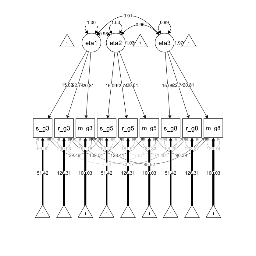
36.2.2. Modello di invarianza debole#
Il modello di invarianza debole impone che la matrice di saturazioni fattoriali sia identica in tutte le occasioni di misurazione. Questo implica che le strutture di covarianza nel tempo siano proporzionali. Tuttavia, il modello permette che le intercette delle variabili osservate possano variare nel tempo e quindi non consente di esaminare il cambiamento longitudinale del fattore.
Definiamo il modello usando la sintassi di lavaan.
weak_invar <- " #opening quote
#factor loadings
  eta1 =~ lambda_S*s_g3+ #removed time-specific subscripts
          lambda_R*r_g3+
          lambda_M*m_g3
  eta2 =~ lambda_S*s_g5+
          lambda_R*r_g5+
          lambda_M*m_g5
  eta3 =~ lambda_S*s_g8+
          lambda_R*r_g8+
          lambda_M*m_g8

#latent variable variances
   eta1~~1*eta1
   eta2~~eta2
   eta3~~eta3

#latent variable covariances
   eta1~~eta2
   eta1~~eta3
   eta2~~eta3

#unique variances
   s_g3~~s_g3
   s_g5~~s_g5
   s_g8~~s_g8
   r_g3~~r_g3
   r_g5~~r_g5
   r_g8~~r_g8
   m_g3~~m_g3
   m_g5~~m_g5
   m_g8~~m_g8
#unique covariances
   s_g3~~s_g5
   s_g3~~s_g8
   s_g5~~s_g8
   r_g3~~r_g5
   r_g3~~r_g8
   r_g5~~r_g8
   m_g3~~m_g5
   m_g3~~m_g8
   m_g5~~m_g8

#latent variable intercepts
   eta1~0*1
   eta2~1
   eta3~1

#observed variable intercepts
   s_g3~tau_S*1
   s_g5~tau_S*1
   s_g8~tau_S*1
   r_g3~tau_R3*1
   r_g5~tau_R5*1
   r_g8~tau_R8*1
   m_g3~tau_M3*1
   m_g5~tau_M5*1
   m_g8~tau_M8*1
" # closing quote
Adattiamo il modello ai dati.
fit_weak <- lavaan(weak_invar, data = dat, mimic = "mplus")
Warning message in lav_data_full(data = data, group = group, cluster = cluster, :
“lavaan WARNING: some cases are empty and will be ignored:
  1 2 5 6 9 11 17 26 37 43 44 53 59 61 65 66 73 77 78 81 90 91 94 95 105 106 108 109 112 115 119 120 125 126 127 129 132 136 137 142 149 150 153 155 156 158 159 160 161 162 164 170 172 176 177 178 180 181 182 183 186 191 192 193 199 206 211 213 218 231 232 237 239 241 260 263 264 271 273 276 279 281 299 300 301 308 310 315 323 324 325 326 327 350 351 352 353 356 362 364 370 372 373 375 376 378 381 386 387 392 393 402 403 404 405 406 409 412 415 420 421 422 429 438 439 443 444 449 455 458 462 464 470 476 478 480 481 483 484 485 486 489 491 494 503 508 518 523 524 541 543 548 552 554 559 561 565 569 573 574 576 579 587 593 595 600 605 607 627 632 642 643 644 646 647 648 663 664 665 666 667 677 680 682 683 687 693 695 698 701 704 713 717 719 720 731 733 734 736 751 755 758 763 764 765 767 768 769 770 772 774 781 782 799 802 818 820 822 827 829 843 846 848 850 857 860 875 878 879 883 891 892 895 897 898 899 900 906 910 911 912 913 915 916 917 918 919 920 923 926 928 929 932 936 938 945 946 948 959 960 964 966 969 970 976 978 980 981 982 983 990 992 993 994 997 998 1002 1005 1009 1016 1022 1025 1035 1043 1044 1045 1047 1054 1056 1057 1061 1062 1080 1087 1088 1090 1095 1096 1098 1099 1104 1105 1106 1107 1109 1113 1115 1117 1118 1125 1126 1127 1128 1129 1131 1133 1139 1146 1149 1152 1153 1157 1163 1164 1165 1167 1172 1183 1185 1186 1195 1198 1200 1202 1211 1215 1218 1228 1229 1236 1238 1247 1248 1249 1250 1251 1252 1255 1259 1262 1263 1264 1266 1267 1270 1275 1276 1277 1279 1280 1281 1286 1289 1290 1302 1303 1306 1309 1310 1311 1314 1317 1320 1329 1330 1336 1338 1339 1343 1344 1353 1354 1356 1357 1358 1360 1367 1372 1379 1384 1386 1389 1399 1403 1405 1410 1411 1412 1414 1418 1421 1422 1423 1428 1429 1430 1434 1437 1439 1441 1445 1449 1451 1455 1459 1462 1464 1465 1466 1467 1469 1471 1480 1483 1487 1488 1493 1496 1497 1506 1507 1516 1528 1530 1531 1533 1534 1535 1536 1537 1538 1543 1544 1545 1549 1553 1555 1556 1557 1558 1559 1562 1565 1568 1570 1573 1579 1580 1581 1586 1587 1593 1594 1597 1601 1602 1605 1606 1610 1612 1615 1620 1622 1626 1629 1634 1636 1638 1648 1654 1657 1659 1662 1663 1669 1670 1671 1672 1681 1682 1685 1686 1687 1688 1690 1699 1702 1705 1706 1710 1712 1717 1719 1720 1727 1728 1729 1736 1742 1745 1748 1751 1762 1765 1766 1771 1777 1778 1780 1787 1788 1789 1790 1794 1796 1797 1804 1809 1822 1826 1828 1831 1836 1838 1839 1840 1841 1844 1845 1846 1854 1855 1860 1862 1863 1865 1866 1867 1869 1874 1875 1876 1878 1879 1885 1886 1891 1895 1897 1899 1902 1903 1906 1911 1914 1915 1916 1924 1925 1926 1930 1931 1933 1943 1944 1950 1954 1959 1960 1964 1965 1969 1978 1980 1985 1986 1990 1993 1994 1996 1997 2000 2004 2008 2009 2010 2012 2013 2014 2016 2017 2019 2021 2029 2030 2031 2032 2033 2034 2035 2043 2045 2050 2051 2052 2053 2056 2061 2066 2069 2073 2075 2076 2079 2080 2090 2101 2102 2105 2108”
Esaminiamo la soluzione.
out = summary(fit_weak, fit.measures = TRUE)
print(out)
lavaan 0.6.15 ended normally after 208 iterations

  Estimator                                         ML
  Optimization method                           NLMINB
  Number of model parameters                        43
  Number of equality constraints                     8

                                                  Used       Total
  Number of observations                          1478        2108
  Number of missing patterns                        24

Model Test User Model:

  Test statistic                               116.826
  Degrees of freedom                                19
  P-value (Chi-square)                           0.000

Model Test Baseline Model:

  Test statistic                             11669.413
  Degrees of freedom                                36
  P-value                                        0.000

User Model versus Baseline Model:

  Comparative Fit Index (CFI)                    0.992
  Tucker-Lewis Index (TLI)                       0.984

  Robust Comparative Fit Index (CFI)             0.991
  Robust Tucker-Lewis Index (TLI)                0.983

Loglikelihood and Information Criteria:

  Loglikelihood user model (H0)             -41958.747
  Loglikelihood unrestricted model (H1)     -41900.334

  Akaike (AIC)                               83987.495
  Bayesian (BIC)                             84172.940
  Sample-size adjusted Bayesian (SABIC)      84061.756

Root Mean Square Error of Approximation:

  RMSEA                                          0.059
  90 Percent confidence interval - lower         0.049
  90 Percent confidence interval - upper         0.070
  P-value H_0: RMSEA <= 0.050                    0.069
  P-value H_0: RMSEA >= 0.080                    0.000

  Robust RMSEA                                   0.071
  90 Percent confidence interval - lower         0.059
  90 Percent confidence interval - upper         0.084
  P-value H_0: Robust RMSEA <= 0.050             0.003
  P-value H_0: Robust RMSEA >= 0.080             0.134

Standardized Root Mean Square Residual:

  SRMR                                           0.062

Parameter Estimates:

  Standard errors                             Standard
  Information                                 Observed
  Observed information based on                Hessian

Latent Variables:
                   Estimate  Std.Err  z-value  P(>|z|)
  eta1 =~
    s_g3    (lm_S)   14.148    0.328   43.128    0.000
    r_g3    (lm_R)   25.418    0.590   43.112    0.000
    m_g3    (lm_M)   20.876    0.524   39.821    0.000
  eta2 =~
    s_g5    (lm_S)   14.148    0.328   43.128    0.000
    r_g5    (lm_R)   25.418    0.590   43.112    0.000
    m_g5    (lm_M)   20.876    0.524   39.821    0.000
  eta3 =~
    s_g8    (lm_S)   14.148    0.328   43.128    0.000
    r_g8    (lm_R)   25.418    0.590   43.112    0.000
    m_g8    (lm_M)   20.876    0.524   39.821    0.000

Covariances:
                   Estimate  Std.Err  z-value  P(>|z|)
  eta1 ~~
    eta2              0.961    0.014   71.113    0.000
    eta3              0.902    0.019   47.928    0.000
  eta2 ~~
    eta3              0.936    0.027   34.664    0.000
 .s_g3 ~~
   .s_g5             33.360    3.070   10.866    0.000
   .s_g8             14.355    3.054    4.700    0.000
 .s_g5 ~~
   .s_g8             22.119    3.248    6.811    0.000
 .r_g3 ~~
   .r_g5             78.937    9.183    8.596    0.000
   .r_g8             52.347    9.433    5.549    0.000
 .r_g5 ~~
   .r_g8             54.402    9.102    5.977    0.000
 .m_g3 ~~
   .m_g5            129.396    8.261   15.664    0.000
   .m_g8             82.602    7.027   11.754    0.000
 .m_g5 ~~
   .m_g8             92.414    7.292   12.673    0.000

Intercepts:
                   Estimate  Std.Err  z-value  P(>|z|)
    eta1              0.000
    eta2              0.977    0.029   33.565    0.000
    eta3              2.293    0.059   38.788    0.000
   .s_g3    (ta_S)   51.012    0.424  120.209    0.000
   .s_g5    (ta_S)   51.012    0.424  120.209    0.000
   .s_g8    (ta_S)   51.012    0.424  120.209    0.000
   .r_g3    (t_R3)  127.284    0.755  168.686    0.000
   .r_g5    (t_R5)  125.448    0.985  127.310    0.000
   .r_g8    (t_R8)  110.884    1.494   74.231    0.000
   .m_g3    (t_M3)   99.743    0.656  152.160    0.000
   .m_g5    (t_M5)  103.390    0.860  120.251    0.000
   .m_g8    (t_M8)   92.568    1.288   71.896    0.000

Variances:
                   Estimate  Std.Err  z-value  P(>|z|)
    eta1              1.000
    eta2              1.000    0.026   37.899    0.000
    eta3              0.979    0.036   27.053    0.000
   .s_g3             63.797    3.533   18.060    0.000
   .s_g5             64.271    3.837   16.751    0.000
   .s_g8             62.052    4.178   14.851    0.000
   .r_g3            187.090   11.494   16.277    0.000
   .r_g5            153.835   10.547   14.585    0.000
   .r_g8            179.482   12.171   14.746    0.000
   .m_g3            194.484    9.513   20.443    0.000
   .m_g5            183.051    9.672   18.926    0.000
   .m_g8            122.637    7.860   15.603    0.000
Generiamo diagramma di percorso.
semPlot::semPaths(
    fit_weak, "std",
    layout = "tree", sizeMan = 7, sizeLat = 7, sizeInt = 4,
    residuals = TRUE, rotation = 1, intAtSide = FALSE,
    whatLabels = "est", nCharNodes = 0, curvature = 3,
    posCol = c("black"), edge.label.cex = .75
)

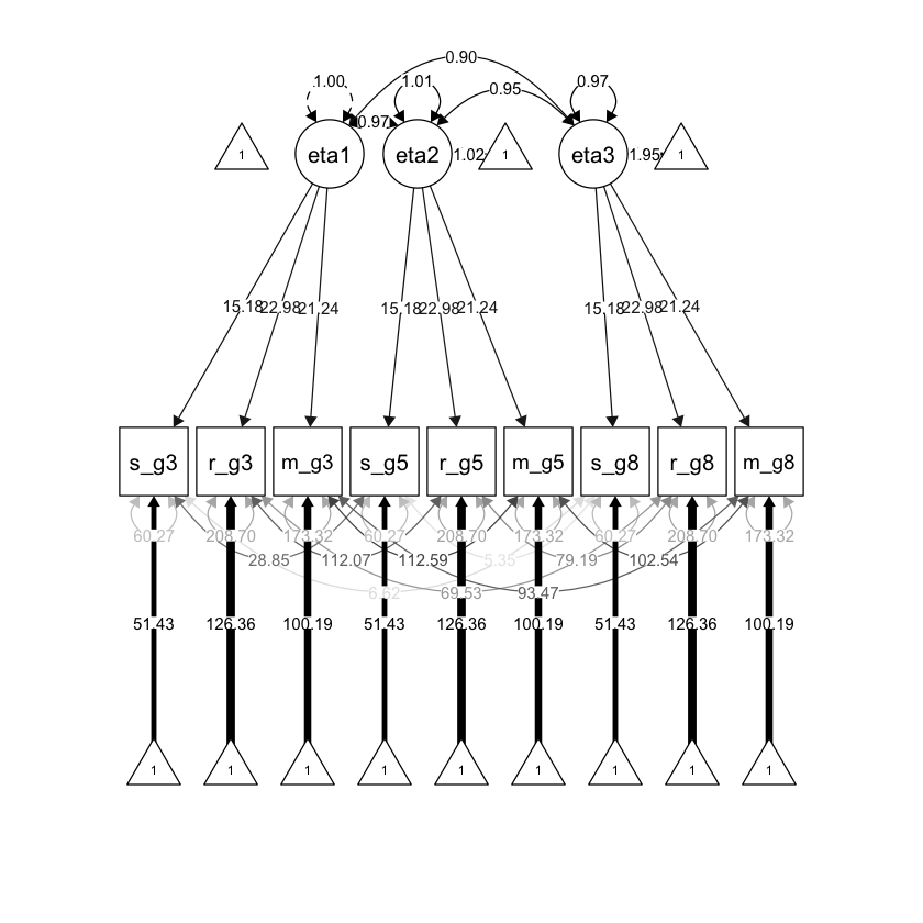
36.2.3. Modello di invarianza forte#
Il modello di invarianza forte impone che le intercette delle variabili osservate siano uguali nel tempo, mentre le medie delle variabili latenti possono variare nelle diverse occasioni. Poiché tutti i cambiamenti nelle medie delle variabili osservate sono attribuiti ai fattori, la scala delle variabili latenti è uguale nelle diverse occasioni di misurazione.
Scriviamo il modello nella sintassi di lavaan.
strong_invar <- " #opening quote
#factor loadings
  eta1 =~ lambda_S*s_g3+ #removed time-specific subscripts
          lambda_R*r_g3+
          lambda_M*m_g3
  eta2 =~ lambda_S*s_g5+
          lambda_R*r_g5+
          lambda_M*m_g5
  eta3 =~ lambda_S*s_g8+
          lambda_R*r_g8+
          lambda_M*m_g8

#latent variable variances
   eta1~~1*eta1
   eta2~~eta2
   eta3~~eta3

#latent variable covariances
   eta1~~eta2
   eta1~~eta3
   eta2~~eta3

#unique variances
   s_g3~~s_g3
   s_g5~~s_g5
   s_g8~~s_g8
   r_g3~~r_g3
   r_g5~~r_g5
   r_g8~~r_g8
   m_g3~~m_g3
   m_g5~~m_g5
   m_g8~~m_g8
#unique covariances
   s_g3~~s_g5
   s_g3~~s_g8
   s_g5~~s_g8
   r_g3~~r_g5
   r_g3~~r_g8
   r_g5~~r_g8
   m_g3~~m_g5
   m_g3~~m_g8
   m_g5~~m_g8

#latent variable intercepts
   eta1~0*1
   eta2~1
   eta3~1

#observed variable intercepts
   s_g3~tau_S*1 #removed time-specific subscripts
   s_g5~tau_S*1
   s_g8~tau_S*1
   r_g3~tau_R*1
   r_g5~tau_R*1
   r_g8~tau_R*1
   m_g3~tau_M*1
   m_g5~tau_M*1
   m_g8~tau_M*1
" # closing quote
Adattiamo il modello ai dati.
fit_strong <- lavaan(strong_invar, data = dat, mimic = "mplus")
Warning message in lav_data_full(data = data, group = group, cluster = cluster, :
“lavaan WARNING: some cases are empty and will be ignored:
  1 2 5 6 9 11 17 26 37 43 44 53 59 61 65 66 73 77 78 81 90 91 94 95 105 106 108 109 112 115 119 120 125 126 127 129 132 136 137 142 149 150 153 155 156 158 159 160 161 162 164 170 172 176 177 178 180 181 182 183 186 191 192 193 199 206 211 213 218 231 232 237 239 241 260 263 264 271 273 276 279 281 299 300 301 308 310 315 323 324 325 326 327 350 351 352 353 356 362 364 370 372 373 375 376 378 381 386 387 392 393 402 403 404 405 406 409 412 415 420 421 422 429 438 439 443 444 449 455 458 462 464 470 476 478 480 481 483 484 485 486 489 491 494 503 508 518 523 524 541 543 548 552 554 559 561 565 569 573 574 576 579 587 593 595 600 605 607 627 632 642 643 644 646 647 648 663 664 665 666 667 677 680 682 683 687 693 695 698 701 704 713 717 719 720 731 733 734 736 751 755 758 763 764 765 767 768 769 770 772 774 781 782 799 802 818 820 822 827 829 843 846 848 850 857 860 875 878 879 883 891 892 895 897 898 899 900 906 910 911 912 913 915 916 917 918 919 920 923 926 928 929 932 936 938 945 946 948 959 960 964 966 969 970 976 978 980 981 982 983 990 992 993 994 997 998 1002 1005 1009 1016 1022 1025 1035 1043 1044 1045 1047 1054 1056 1057 1061 1062 1080 1087 1088 1090 1095 1096 1098 1099 1104 1105 1106 1107 1109 1113 1115 1117 1118 1125 1126 1127 1128 1129 1131 1133 1139 1146 1149 1152 1153 1157 1163 1164 1165 1167 1172 1183 1185 1186 1195 1198 1200 1202 1211 1215 1218 1228 1229 1236 1238 1247 1248 1249 1250 1251 1252 1255 1259 1262 1263 1264 1266 1267 1270 1275 1276 1277 1279 1280 1281 1286 1289 1290 1302 1303 1306 1309 1310 1311 1314 1317 1320 1329 1330 1336 1338 1339 1343 1344 1353 1354 1356 1357 1358 1360 1367 1372 1379 1384 1386 1389 1399 1403 1405 1410 1411 1412 1414 1418 1421 1422 1423 1428 1429 1430 1434 1437 1439 1441 1445 1449 1451 1455 1459 1462 1464 1465 1466 1467 1469 1471 1480 1483 1487 1488 1493 1496 1497 1506 1507 1516 1528 1530 1531 1533 1534 1535 1536 1537 1538 1543 1544 1545 1549 1553 1555 1556 1557 1558 1559 1562 1565 1568 1570 1573 1579 1580 1581 1586 1587 1593 1594 1597 1601 1602 1605 1606 1610 1612 1615 1620 1622 1626 1629 1634 1636 1638 1648 1654 1657 1659 1662 1663 1669 1670 1671 1672 1681 1682 1685 1686 1687 1688 1690 1699 1702 1705 1706 1710 1712 1717 1719 1720 1727 1728 1729 1736 1742 1745 1748 1751 1762 1765 1766 1771 1777 1778 1780 1787 1788 1789 1790 1794 1796 1797 1804 1809 1822 1826 1828 1831 1836 1838 1839 1840 1841 1844 1845 1846 1854 1855 1860 1862 1863 1865 1866 1867 1869 1874 1875 1876 1878 1879 1885 1886 1891 1895 1897 1899 1902 1903 1906 1911 1914 1915 1916 1924 1925 1926 1930 1931 1933 1943 1944 1950 1954 1959 1960 1964 1965 1969 1978 1980 1985 1986 1990 1993 1994 1996 1997 2000 2004 2008 2009 2010 2012 2013 2014 2016 2017 2019 2021 2029 2030 2031 2032 2033 2034 2035 2043 2045 2050 2051 2052 2053 2056 2061 2066 2069 2073 2075 2076 2079 2080 2090 2101 2102 2105 2108”
Esaminiamo la soluzione.
out = summary(fit_strong, fit.measures = TRUE)
print(out)
lavaan 0.6.15 ended normally after 218 iterations

  Estimator                                         ML
  Optimization method                           NLMINB
  Number of model parameters                        43
  Number of equality constraints                    12

                                                  Used       Total
  Number of observations                          1478        2108
  Number of missing patterns                        24

Model Test User Model:

  Test statistic                               540.750
  Degrees of freedom                                23
  P-value (Chi-square)                           0.000

Model Test Baseline Model:

  Test statistic                             11669.413
  Degrees of freedom                                36
  P-value                                        0.000

User Model versus Baseline Model:

  Comparative Fit Index (CFI)                    0.955
  Tucker-Lewis Index (TLI)                       0.930

  Robust Comparative Fit Index (CFI)             0.957
  Robust Tucker-Lewis Index (TLI)                0.932

Loglikelihood and Information Criteria:

  Loglikelihood user model (H0)             -42170.709
  Loglikelihood unrestricted model (H1)     -41900.334

  Akaike (AIC)                               84403.419
  Bayesian (BIC)                             84567.670
  Sample-size adjusted Bayesian (SABIC)      84469.193

Root Mean Square Error of Approximation:

  RMSEA                                          0.123
  90 Percent confidence interval - lower         0.115
  90 Percent confidence interval - upper         0.133
  P-value H_0: RMSEA <= 0.050                    0.000
  P-value H_0: RMSEA >= 0.080                    1.000

  Robust RMSEA                                   0.142
  90 Percent confidence interval - lower         0.132
  90 Percent confidence interval - upper         0.154
  P-value H_0: Robust RMSEA <= 0.050             0.000
  P-value H_0: Robust RMSEA >= 0.080             1.000

Standardized Root Mean Square Residual:

  SRMR                                           0.096

Parameter Estimates:

  Standard errors                             Standard
  Information                                 Observed
  Observed information based on                Hessian

Latent Variables:
                   Estimate  Std.Err  z-value  P(>|z|)
  eta1 =~
    s_g3    (lm_S)   15.088    0.322   46.858    0.000
    r_g3    (lm_R)   22.740    0.524   43.414    0.000
    m_g3    (lm_M)   20.807    0.473   44.030    0.000
  eta2 =~
    s_g5    (lm_S)   15.088    0.322   46.858    0.000
    r_g5    (lm_R)   22.740    0.524   43.414    0.000
    m_g5    (lm_M)   20.807    0.473   44.030    0.000
  eta3 =~
    s_g8    (lm_S)   15.088    0.322   46.858    0.000
    r_g8    (lm_R)   22.740    0.524   43.414    0.000
    m_g8    (lm_M)   20.807    0.473   44.030    0.000

Covariances:
                   Estimate  Std.Err  z-value  P(>|z|)
  eta1 ~~
    eta2              0.976    0.014   70.707    0.000
    eta3              0.910    0.019   47.377    0.000
  eta2 ~~
    eta3              0.961    0.028   34.465    0.000
 .s_g3 ~~
   .s_g5             29.487    3.487    8.456    0.000
   .s_g8              7.394    3.251    2.274    0.023
 .s_g5 ~~
   .s_g8              7.867    3.332    2.361    0.018
 .r_g3 ~~
   .r_g5            109.044    9.413   11.585    0.000
   .r_g8             73.172    9.982    7.330    0.000
 .r_g5 ~~
   .r_g8             71.480    9.209    7.762    0.000
 .m_g3 ~~
   .m_g5            128.408    8.511   15.088    0.000
   .m_g8             85.516    7.421   11.523    0.000
 .m_g5 ~~
   .m_g8             90.389    7.594   11.903    0.000

Intercepts:
                   Estimate  Std.Err  z-value  P(>|z|)
    eta1              0.000
    eta2              1.032    0.026   40.382    0.000
    eta3              1.972    0.046   42.668    0.000
   .s_g3    (ta_S)   51.422    0.450  114.287    0.000
   .s_g5    (ta_S)   51.422    0.450  114.287    0.000
   .s_g8    (ta_S)   51.422    0.450  114.287    0.000
   .r_g3    (ta_R)  126.310    0.706  179.023    0.000
   .r_g5    (ta_R)  126.310    0.706  179.023    0.000
   .r_g8    (ta_R)  126.310    0.706  179.023    0.000
   .m_g3    (ta_M)  100.035    0.658  152.097    0.000
   .m_g5    (ta_M)  100.035    0.658  152.097    0.000
   .m_g8    (ta_M)  100.035    0.658  152.097    0.000

Variances:
                   Estimate  Std.Err  z-value  P(>|z|)
    eta1              1.000
    eta2              1.025    0.027   37.549    0.000
    eta3              0.990    0.037   26.783    0.000
   .s_g3             58.999    3.875   15.224    0.000
   .s_g5             63.402    4.314   14.698    0.000
   .s_g8             58.256    4.688   12.427    0.000
   .r_g3            230.033   11.800   19.494    0.000
   .r_g5            181.922   10.581   17.193    0.000
   .r_g8            208.269   12.238   17.019    0.000
   .m_g3            197.179    9.868   19.981    0.000
   .m_g5            188.328   10.123   18.603    0.000
   .m_g8            126.741    8.199   15.458    0.000
Generiamo il diagramma di percorso.
semPlot::semPaths(
    fit_strong, "std",
    layout = "tree", sizeMan = 7, sizeLat = 7, sizeInt = 4,
    residuals = TRUE, rotation = 1, intAtSide = FALSE,
    whatLabels = "est", nCharNodes = 0, curvature = 3,
    posCol = c("black"), edge.label.cex = .75
)
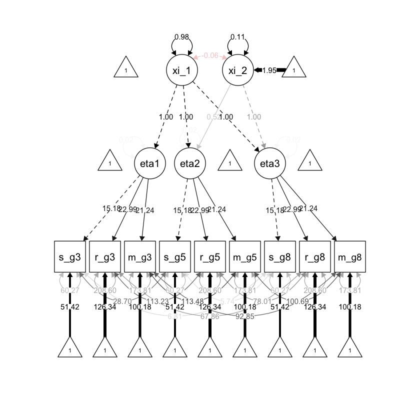
36.2.4. Invarianza stretta#
Il modello di invarianza rigorosa impone vincoli aggiuntivi sulle saturazioni fattoriali, sulle intercette delle variabili osservate e sulle varianze uniche. Quando l’invarianza fattoriale rigorosa è soddisfatta, i cambiamenti longitudinali nelle medie osservate, nelle varianze e nelle covarianze ci informano sui cambiamenti longitudinali dei fattori.
Definiamo il modello con la sintassi di lavaan.
strict_invar <- " #opening quote
#factor loadings
  eta1 =~ lambda_S*s_g3+ #removed time-specific subscripts
          lambda_R*r_g3+
          lambda_M*m_g3
  eta2 =~ lambda_S*s_g5+
          lambda_R*r_g5+
          lambda_M*m_g5
  eta3 =~ lambda_S*s_g8+
          lambda_R*r_g8+
          lambda_M*m_g8

#latent variable variances
   eta1~~1*eta1
   eta2~~eta2
   eta3~~eta3

#latent variable covariances
   eta1~~eta2
   eta1~~eta3
   eta2~~eta3

#unique variances
   s_g3~~theta_S*s_g3 #adding constraints with names
   s_g5~~theta_S*s_g5
   s_g8~~theta_S*s_g8
   r_g3~~theta_R*r_g3
   r_g5~~theta_R*r_g5
   r_g8~~theta_R*r_g8
   m_g3~~theta_M*m_g3
   m_g5~~theta_M*m_g5
   m_g8~~theta_M*m_g8
#unique covariances
   s_g3~~s_g5
   s_g3~~s_g8
   s_g5~~s_g8
   r_g3~~r_g5
   r_g3~~r_g8
   r_g5~~r_g8
   m_g3~~m_g5
   m_g3~~m_g8
   m_g5~~m_g8

#latent variable intercepts
   eta1~0*1
   eta2~1
   eta3~1

#observed variable intercepts
   s_g3~tau_S*1 #removed time-specific subscripts
   s_g5~tau_S*1
   s_g8~tau_S*1
   r_g3~tau_R*1
   r_g5~tau_R*1
   r_g8~tau_R*1
   m_g3~tau_M*1
   m_g5~tau_M*1
   m_g8~tau_M*1
" # closing quote
Adattiamo il modello ai dati.
fit_strict <- lavaan(strict_invar, data = dat, mimic = "mplus")
Warning message in lav_data_full(data = data, group = group, cluster = cluster, :
“lavaan WARNING: some cases are empty and will be ignored:
  1 2 5 6 9 11 17 26 37 43 44 53 59 61 65 66 73 77 78 81 90 91 94 95 105 106 108 109 112 115 119 120 125 126 127 129 132 136 137 142 149 150 153 155 156 158 159 160 161 162 164 170 172 176 177 178 180 181 182 183 186 191 192 193 199 206 211 213 218 231 232 237 239 241 260 263 264 271 273 276 279 281 299 300 301 308 310 315 323 324 325 326 327 350 351 352 353 356 362 364 370 372 373 375 376 378 381 386 387 392 393 402 403 404 405 406 409 412 415 420 421 422 429 438 439 443 444 449 455 458 462 464 470 476 478 480 481 483 484 485 486 489 491 494 503 508 518 523 524 541 543 548 552 554 559 561 565 569 573 574 576 579 587 593 595 600 605 607 627 632 642 643 644 646 647 648 663 664 665 666 667 677 680 682 683 687 693 695 698 701 704 713 717 719 720 731 733 734 736 751 755 758 763 764 765 767 768 769 770 772 774 781 782 799 802 818 820 822 827 829 843 846 848 850 857 860 875 878 879 883 891 892 895 897 898 899 900 906 910 911 912 913 915 916 917 918 919 920 923 926 928 929 932 936 938 945 946 948 959 960 964 966 969 970 976 978 980 981 982 983 990 992 993 994 997 998 1002 1005 1009 1016 1022 1025 1035 1043 1044 1045 1047 1054 1056 1057 1061 1062 1080 1087 1088 1090 1095 1096 1098 1099 1104 1105 1106 1107 1109 1113 1115 1117 1118 1125 1126 1127 1128 1129 1131 1133 1139 1146 1149 1152 1153 1157 1163 1164 1165 1167 1172 1183 1185 1186 1195 1198 1200 1202 1211 1215 1218 1228 1229 1236 1238 1247 1248 1249 1250 1251 1252 1255 1259 1262 1263 1264 1266 1267 1270 1275 1276 1277 1279 1280 1281 1286 1289 1290 1302 1303 1306 1309 1310 1311 1314 1317 1320 1329 1330 1336 1338 1339 1343 1344 1353 1354 1356 1357 1358 1360 1367 1372 1379 1384 1386 1389 1399 1403 1405 1410 1411 1412 1414 1418 1421 1422 1423 1428 1429 1430 1434 1437 1439 1441 1445 1449 1451 1455 1459 1462 1464 1465 1466 1467 1469 1471 1480 1483 1487 1488 1493 1496 1497 1506 1507 1516 1528 1530 1531 1533 1534 1535 1536 1537 1538 1543 1544 1545 1549 1553 1555 1556 1557 1558 1559 1562 1565 1568 1570 1573 1579 1580 1581 1586 1587 1593 1594 1597 1601 1602 1605 1606 1610 1612 1615 1620 1622 1626 1629 1634 1636 1638 1648 1654 1657 1659 1662 1663 1669 1670 1671 1672 1681 1682 1685 1686 1687 1688 1690 1699 1702 1705 1706 1710 1712 1717 1719 1720 1727 1728 1729 1736 1742 1745 1748 1751 1762 1765 1766 1771 1777 1778 1780 1787 1788 1789 1790 1794 1796 1797 1804 1809 1822 1826 1828 1831 1836 1838 1839 1840 1841 1844 1845 1846 1854 1855 1860 1862 1863 1865 1866 1867 1869 1874 1875 1876 1878 1879 1885 1886 1891 1895 1897 1899 1902 1903 1906 1911 1914 1915 1916 1924 1925 1926 1930 1931 1933 1943 1944 1950 1954 1959 1960 1964 1965 1969 1978 1980 1985 1986 1990 1993 1994 1996 1997 2000 2004 2008 2009 2010 2012 2013 2014 2016 2017 2019 2021 2029 2030 2031 2032 2033 2034 2035 2043 2045 2050 2051 2052 2053 2056 2061 2066 2069 2073 2075 2076 2079 2080 2090 2101 2102 2105 2108”
Esaminiamo la soluzione ottenuta.
out = summary(fit_strict, fit.measures = TRUE)
print(out)
lavaan 0.6.15 ended normally after 260 iterations

  Estimator                                         ML
  Optimization method                           NLMINB
  Number of model parameters                        43
  Number of equality constraints                    18

                                                  Used       Total
  Number of observations                          1478        2108
  Number of missing patterns                        24

Model Test User Model:

  Test statistic                               600.614
  Degrees of freedom                                29
  P-value (Chi-square)                           0.000

Model Test Baseline Model:

  Test statistic                             11669.413
  Degrees of freedom                                36
  P-value                                        0.000

User Model versus Baseline Model:

  Comparative Fit Index (CFI)                    0.951
  Tucker-Lewis Index (TLI)                       0.939

  Robust Comparative Fit Index (CFI)             0.952
  Robust Tucker-Lewis Index (TLI)                0.940

Loglikelihood and Information Criteria:

  Loglikelihood user model (H0)             -42200.641
  Loglikelihood unrestricted model (H1)     -41900.334

  Akaike (AIC)                               84451.282
  Bayesian (BIC)                             84583.743
  Sample-size adjusted Bayesian (SABIC)      84504.325

Root Mean Square Error of Approximation:

  RMSEA                                          0.115
  90 Percent confidence interval - lower         0.108
  90 Percent confidence interval - upper         0.124
  P-value H_0: RMSEA <= 0.050                    0.000
  P-value H_0: RMSEA >= 0.080                    1.000

  Robust RMSEA                                   0.134
  90 Percent confidence interval - lower         0.125
  90 Percent confidence interval - upper         0.144
  P-value H_0: Robust RMSEA <= 0.050             0.000
  P-value H_0: Robust RMSEA >= 0.080             1.000

Standardized Root Mean Square Residual:

  SRMR                                           0.111

Parameter Estimates:

  Standard errors                             Standard
  Information                                 Observed
  Observed information based on                Hessian

Latent Variables:
                   Estimate  Std.Err  z-value  P(>|z|)
  eta1 =~
    s_g3    (lm_S)   15.176    0.319   47.527    0.000
    r_g3    (lm_R)   22.982    0.520   44.172    0.000
    m_g3    (lm_M)   21.236    0.473   44.918    0.000
  eta2 =~
    s_g5    (lm_S)   15.176    0.319   47.527    0.000
    r_g5    (lm_R)   22.982    0.520   44.172    0.000
    m_g5    (lm_M)   21.236    0.473   44.918    0.000
  eta3 =~
    s_g8    (lm_S)   15.176    0.319   47.527    0.000
    r_g8    (lm_R)   22.982    0.520   44.172    0.000
    m_g8    (lm_M)   21.236    0.473   44.918    0.000

Covariances:
                   Estimate  Std.Err  z-value  P(>|z|)
  eta1 ~~
    eta2              0.968    0.013   72.280    0.000
    eta3              0.904    0.019   48.240    0.000
  eta2 ~~
    eta3              0.949    0.027   35.094    0.000
 .s_g3 ~~
   .s_g5             28.853    3.118    9.254    0.000
   .s_g8              6.616    3.301    2.004    0.045
 .s_g5 ~~
   .s_g8              5.354    3.311    1.617    0.106
 .r_g3 ~~
   .r_g5            112.069    8.673   12.921    0.000
   .r_g8             69.529    9.345    7.440    0.000
 .r_g5 ~~
   .r_g8             79.188    9.640    8.214    0.000
 .m_g3 ~~
   .m_g5            112.589    7.308   15.407    0.000
   .m_g8             93.467    7.990   11.698    0.000
 .m_g5 ~~
   .m_g8            102.538    8.014   12.794    0.000

Intercepts:
                   Estimate  Std.Err  z-value  P(>|z|)
    eta1              0.000
    eta2              1.020    0.025   41.017    0.000
    eta3              1.947    0.045   43.249    0.000
   .s_g3    (ta_S)   51.433    0.448  114.745    0.000
   .s_g5    (ta_S)   51.433    0.448  114.745    0.000
   .s_g8    (ta_S)   51.433    0.448  114.745    0.000
   .r_g3    (ta_R)  126.363    0.702  179.899    0.000
   .r_g5    (ta_R)  126.363    0.702  179.899    0.000
   .r_g8    (ta_R)  126.363    0.702  179.899    0.000
   .m_g3    (ta_M)  100.193    0.651  153.913    0.000
   .m_g5    (ta_M)  100.193    0.651  153.913    0.000
   .m_g8    (ta_M)  100.193    0.651  153.913    0.000

Variances:
                   Estimate  Std.Err  z-value  P(>|z|)
    eta1              1.000
    eta2              1.011    0.026   38.332    0.000
    eta3              0.971    0.036   27.168    0.000
   .s_g3    (th_S)   60.274    2.939   20.506    0.000
   .s_g5    (th_S)   60.274    2.939   20.506    0.000
   .s_g8    (th_S)   60.274    2.939   20.506    0.000
   .r_g3    (th_R)  208.701    8.172   25.537    0.000
   .r_g5    (th_R)  208.701    8.172   25.537    0.000
   .r_g8    (th_R)  208.701    8.172   25.537    0.000
   .m_g3    (th_M)  173.321    7.236   23.952    0.000
   .m_g5    (th_M)  173.321    7.236   23.952    0.000
   .m_g8    (th_M)  173.321    7.236   23.952    0.000
Generiamo il diagramma di percorso.
semPlot::semPaths(
    fit_strict, "std",
    layout = "tree", sizeMan = 7, sizeLat = 7, sizeInt = 4,
    residuals = TRUE, rotation = 1, intAtSide = FALSE,
    whatLabels = "est", nCharNodes = 0, curvature = 3,
    posCol = c("black"), edge.label.cex = .75
)
36.3. Confronto tra modelli#
È possibile valutare il tipo di invarianza fattoriale longitudinale giustificata dai dati mediante un confronto tra modelli.
round(cbind(
  configural = inspect(fit_configural, "fit.measures"),
  weak = inspect(fit_weak, "fit.measures"),
  strong = inspect(fit_strong, "fit.measures"),
  strict = inspect(fit_strict, "fit.measures")
), 3)
| configural | weak | strong | strict | |
|---|---|---|---|---|
| npar | 39.000 | 35.000 | 31.000 | 25.000 |
| fmin | 0.012 | 0.040 | 0.183 | 0.203 |
| chisq | 35.522 | 116.826 | 540.750 | 600.614 |
| df | 15.000 | 19.000 | 23.000 | 29.000 |
| pvalue | 0.002 | 0.000 | 0.000 | 0.000 |
| baseline.chisq | 11669.413 | 11669.413 | 11669.413 | 11669.413 |
| baseline.df | 36.000 | 36.000 | 36.000 | 36.000 |
| baseline.pvalue | 0.000 | 0.000 | 0.000 | 0.000 |
| cfi | 0.998 | 0.992 | 0.955 | 0.951 |
| tli | 0.996 | 0.984 | 0.930 | 0.939 |
| cfi.robust | 0.998 | 0.991 | 0.957 | 0.952 |
| tli.robust | 0.995 | 0.983 | 0.932 | 0.940 |
| nnfi | 0.996 | 0.984 | 0.930 | 0.939 |
| rfi | 0.993 | 0.981 | 0.927 | 0.936 |
| nfi | 0.997 | 0.990 | 0.954 | 0.949 |
| pnfi | 0.415 | 0.522 | 0.609 | 0.764 |
| ifi | 0.998 | 0.992 | 0.956 | 0.951 |
| rni | 0.998 | 0.992 | 0.955 | 0.951 |
| nnfi.robust | 0.995 | 0.983 | 0.932 | 0.940 |
| rni.robust | 0.998 | 0.991 | 0.957 | 0.952 |
| logl | -41918.095 | -41958.747 | -42170.709 | -42200.641 |
| unrestricted.logl | -41900.334 | -41900.334 | -41900.334 | -41900.334 |
| aic | 83914.190 | 83987.495 | 84403.419 | 84451.282 |
| bic | 84120.830 | 84172.940 | 84567.670 | 84583.743 |
| ntotal | 1478.000 | 1478.000 | 1478.000 | 1478.000 |
| bic2 | 83996.938 | 84061.756 | 84469.193 | 84504.325 |
| rmsea | 0.030 | 0.059 | 0.123 | 0.115 |
| rmsea.ci.lower | 0.018 | 0.049 | 0.115 | 0.108 |
| rmsea.ci.upper | 0.043 | 0.070 | 0.133 | 0.124 |
| rmsea.ci.level | 0.900 | 0.900 | 0.900 | 0.900 |
| rmsea.pvalue | 0.994 | 0.069 | 0.000 | 0.000 |
| rmsea.close.h0 | 0.050 | 0.050 | 0.050 | 0.050 |
| rmsea.notclose.pvalue | 0.000 | 0.000 | 1.000 | 1.000 |
| rmsea.notclose.h0 | 0.080 | 0.080 | 0.080 | 0.080 |
| rmsea.robust | 0.037 | 0.071 | 0.142 | 0.134 |
| rmsea.ci.lower.robust | 0.021 | 0.059 | 0.132 | 0.125 |
| rmsea.ci.upper.robust | 0.053 | 0.084 | 0.154 | 0.144 |
| rmsea.pvalue.robust | 0.897 | 0.003 | 0.000 | 0.000 |
| rmsea.notclose.pvalue.robust | 0.000 | 0.134 | 1.000 | 1.000 |
| rmr | 3.876 | 20.127 | 41.365 | 40.928 |
| rmr_nomean | 4.246 | 22.048 | 45.308 | 44.829 |
| srmr | 0.008 | 0.062 | 0.096 | 0.111 |
| srmr_bentler | 0.007 | 0.042 | 0.075 | 0.078 |
| srmr_bentler_nomean | 0.008 | 0.046 | 0.076 | 0.079 |
| crmr | 0.008 | 0.016 | 0.042 | 0.041 |
| crmr_nomean | 0.009 | 0.018 | 0.028 | 0.027 |
| srmr_mplus | 0.008 | 0.062 | 0.096 | 0.111 |
| srmr_mplus_nomean | 0.008 | 0.030 | 0.050 | 0.055 |
| cn_05 | 1041.031 | 382.354 | 97.135 | 105.725 |
| cn_01 | 1273.294 | 458.860 | 114.808 | 123.027 |
| gfi | 0.997 | 0.996 | 0.991 | 0.990 |
| agfi | 0.990 | 0.989 | 0.980 | 0.982 |
| pgfi | 0.277 | 0.350 | 0.422 | 0.532 |
| mfi | 0.993 | 0.967 | 0.839 | 0.824 |
| ecvi | 0.077 | 0.126 | 0.408 | 0.440 |
# Chi-square difference test for nested models
lavTestLRT(fit_configural, fit_weak) |>
    print()
Chi-Squared Difference Test

               Df   AIC   BIC   Chisq Chisq diff   RMSEA Df diff Pr(>Chisq)
fit_configural 15 83914 84121  35.522
fit_weak       19 83987 84173 116.826     81.304 0.11435       4  < 2.2e-16 ***
---
Signif. codes:  0 ‘***’ 0.001 ‘**’ 0.01 ‘*’ 0.05 ‘.’ 0.1 ‘ ’ 1
lavTestLRT(fit_weak, fit_strong) |>
    print()
Chi-Squared Difference Test

           Df   AIC   BIC  Chisq Chisq diff   RMSEA Df diff Pr(>Chisq)
fit_weak   19 83987 84173 116.83
fit_strong 23 84403 84568 540.75     423.92 0.26651       4  < 2.2e-16 ***
---
Signif. codes:  0 ‘***’ 0.001 ‘**’ 0.01 ‘*’ 0.05 ‘.’ 0.1 ‘ ’ 1
lavTestLRT(fit_strong, fit_strict) |>
    print()
Chi-Squared Difference Test

           Df   AIC   BIC  Chisq Chisq diff    RMSEA Df diff Pr(>Chisq)
fit_strong 23 84403 84568 540.75
fit_strict 29 84451 84584 600.61     59.863 0.077935       6  4.798e-11 ***
---
Signif. codes:  0 ‘***’ 0.001 ‘**’ 0.01 ‘*’ 0.05 ‘.’ 0.1 ‘ ’ 1
Nel caso presente, solo l’invarianza configurale è giustificata dal test di verosimiglianze. L’esame degli indici di bontà di adattamento, comunque, suggerisce che l’invarianza debole sembra giustificata per questi dati. @grimm2016growth concludono invece che anche l’invarianza forte è giustificata per questi dati.
36.4. Second-Order Growth Model#
Una volta che abbiamo dimostrato che l’invarianza forte o rigorosa è supportata per il modello di crescita latente, possiamo esaminare i cambiamenti nei punteggi fattoriali.
In questo esempio, imponiamo l’invarianza fattoriale rigorosa e modelliamo il cambiamento nei punteggi fattoriali del rendimento accademico dei bambini utilizzando un Second-Order Growth Model. Si noti che devono essere apportate alcune altre modifiche per l’identificazione e la scala.
growth_strict_invar <- " #opening quote
#factor loadings
  eta1 =~ 15.176*s_g3+ #constrained for identification and scaling
          lambda_R*r_g3+
          lambda_M*m_g3
  eta2 =~ 15.176*s_g5+
          lambda_R*r_g5+
          lambda_M*m_g5
  eta3 =~ 15.176*s_g8+
          lambda_R*r_g8+
          lambda_M*m_g8

#latent variable variances
   eta1~~psi*eta1
   eta2~~psi*eta2
   eta3~~psi*eta3

#latent variable covariances
   eta1~~0*eta2 #constrained to zero
   eta1~~0*eta3
   eta2~~0*eta3

#unique variances
   s_g3~~theta_S*s_g3 #adding constraints with names
   s_g5~~theta_S*s_g5
   s_g8~~theta_S*s_g8
   r_g3~~theta_R*r_g3
   r_g5~~theta_R*r_g5
   r_g8~~theta_R*r_g8
   m_g3~~theta_M*m_g3
   m_g5~~theta_M*m_g5
   m_g8~~theta_M*m_g8
#unique covariances
   s_g3~~s_g5
   s_g3~~s_g8
   s_g5~~s_g8
   r_g3~~r_g5
   r_g3~~r_g8
   r_g5~~r_g8
   m_g3~~m_g5
   m_g3~~m_g8
   m_g5~~m_g8

#latent variable intercepts
   eta1~0*1  #fixed to zero
   eta2~0*1
   eta3~0*1

#observed variable intercepts
   s_g3~tau_S*1 #removed time-specific subscripts
   s_g5~tau_S*1
   s_g8~tau_S*1
   r_g3~tau_R*1
   r_g5~tau_R*1
   r_g8~tau_R*1
   m_g3~tau_M*1
   m_g5~tau_M*1
   m_g8~tau_M*1

#second-order latent basis growth
  #growth factors
   xi_1 =~ 1*eta1+ #intercept factor
           1*eta2+
           1*eta3
   xi_2 =~ 0*eta1  #latent basis slope factor
           +start(0.5)*eta2
           +1*eta3
  #factor variances & covariance
    xi_1~~start(.8)*xi_1
    xi_2~~start(.5)*xi_2
    xi_1~~start(0)*xi_2
  #factor intercepts
    xi_1~0*1
    xi_2~1
" # closing quote
Adattiamo il modello ai dati.
fit_growth <- lavaan(growth_strict_invar, data = dat, mimic = "mplus")
Warning message in lav_data_full(data = data, group = group, cluster = cluster, :
“lavaan WARNING: some cases are empty and will be ignored:
  1 2 5 6 9 11 17 26 37 43 44 53 59 61 65 66 73 77 78 81 90 91 94 95 105 106 108 109 112 115 119 120 125 126 127 129 132 136 137 142 149 150 153 155 156 158 159 160 161 162 164 170 172 176 177 178 180 181 182 183 186 191 192 193 199 206 211 213 218 231 232 237 239 241 260 263 264 271 273 276 279 281 299 300 301 308 310 315 323 324 325 326 327 350 351 352 353 356 362 364 370 372 373 375 376 378 381 386 387 392 393 402 403 404 405 406 409 412 415 420 421 422 429 438 439 443 444 449 455 458 462 464 470 476 478 480 481 483 484 485 486 489 491 494 503 508 518 523 524 541 543 548 552 554 559 561 565 569 573 574 576 579 587 593 595 600 605 607 627 632 642 643 644 646 647 648 663 664 665 666 667 677 680 682 683 687 693 695 698 701 704 713 717 719 720 731 733 734 736 751 755 758 763 764 765 767 768 769 770 772 774 781 782 799 802 818 820 822 827 829 843 846 848 850 857 860 875 878 879 883 891 892 895 897 898 899 900 906 910 911 912 913 915 916 917 918 919 920 923 926 928 929 932 936 938 945 946 948 959 960 964 966 969 970 976 978 980 981 982 983 990 992 993 994 997 998 1002 1005 1009 1016 1022 1025 1035 1043 1044 1045 1047 1054 1056 1057 1061 1062 1080 1087 1088 1090 1095 1096 1098 1099 1104 1105 1106 1107 1109 1113 1115 1117 1118 1125 1126 1127 1128 1129 1131 1133 1139 1146 1149 1152 1153 1157 1163 1164 1165 1167 1172 1183 1185 1186 1195 1198 1200 1202 1211 1215 1218 1228 1229 1236 1238 1247 1248 1249 1250 1251 1252 1255 1259 1262 1263 1264 1266 1267 1270 1275 1276 1277 1279 1280 1281 1286 1289 1290 1302 1303 1306 1309 1310 1311 1314 1317 1320 1329 1330 1336 1338 1339 1343 1344 1353 1354 1356 1357 1358 1360 1367 1372 1379 1384 1386 1389 1399 1403 1405 1410 1411 1412 1414 1418 1421 1422 1423 1428 1429 1430 1434 1437 1439 1441 1445 1449 1451 1455 1459 1462 1464 1465 1466 1467 1469 1471 1480 1483 1487 1488 1493 1496 1497 1506 1507 1516 1528 1530 1531 1533 1534 1535 1536 1537 1538 1543 1544 1545 1549 1553 1555 1556 1557 1558 1559 1562 1565 1568 1570 1573 1579 1580 1581 1586 1587 1593 1594 1597 1601 1602 1605 1606 1610 1612 1615 1620 1622 1626 1629 1634 1636 1638 1648 1654 1657 1659 1662 1663 1669 1670 1671 1672 1681 1682 1685 1686 1687 1688 1690 1699 1702 1705 1706 1710 1712 1717 1719 1720 1727 1728 1729 1736 1742 1745 1748 1751 1762 1765 1766 1771 1777 1778 1780 1787 1788 1789 1790 1794 1796 1797 1804 1809 1822 1826 1828 1831 1836 1838 1839 1840 1841 1844 1845 1846 1854 1855 1860 1862 1863 1865 1866 1867 1869 1874 1875 1876 1878 1879 1885 1886 1891 1895 1897 1899 1902 1903 1906 1911 1914 1915 1916 1924 1925 1926 1930 1931 1933 1943 1944 1950 1954 1959 1960 1964 1965 1969 1978 1980 1985 1986 1990 1993 1994 1996 1997 2000 2004 2008 2009 2010 2012 2013 2014 2016 2017 2019 2021 2029 2030 2031 2032 2033 2034 2035 2043 2045 2050 2051 2052 2053 2056 2061 2066 2069 2073 2075 2076 2079 2080 2090 2101 2102 2105 2108”
Esaminiamo la soluzione.
out = summary(fit_growth, fit.measures = TRUE)
print(out)
lavaan 0.6.15 ended normally after 192 iterations

  Estimator                                         ML
  Optimization method                           NLMINB
  Number of model parameters                        41
  Number of equality constraints                    18

                                                  Used       Total
  Number of observations                          1478        2108
  Number of missing patterns                        24

Model Test User Model:

  Test statistic                               606.985
  Degrees of freedom                                31
  P-value (Chi-square)                           0.000

Model Test Baseline Model:

  Test statistic                             11669.413
  Degrees of freedom                                36
  P-value                                        0.000

User Model versus Baseline Model:

  Comparative Fit Index (CFI)                    0.950
  Tucker-Lewis Index (TLI)                       0.943

  Robust Comparative Fit Index (CFI)             0.951
  Robust Tucker-Lewis Index (TLI)                0.943

Loglikelihood and Information Criteria:

  Loglikelihood user model (H0)             -42203.827
  Loglikelihood unrestricted model (H1)     -41900.334

  Akaike (AIC)                               84453.654
  Bayesian (BIC)                             84575.518
  Sample-size adjusted Bayesian (SABIC)      84502.454

Root Mean Square Error of Approximation:

  RMSEA                                          0.112
  90 Percent confidence interval - lower         0.104
  90 Percent confidence interval - upper         0.120
  P-value H_0: RMSEA <= 0.050                    0.000
  P-value H_0: RMSEA >= 0.080                    1.000

  Robust RMSEA                                   0.131
  90 Percent confidence interval - lower         0.121
  90 Percent confidence interval - upper         0.140
  P-value H_0: Robust RMSEA <= 0.050             0.000
  P-value H_0: Robust RMSEA >= 0.080             1.000

Standardized Root Mean Square Residual:

  SRMR                                           0.113

Parameter Estimates:

  Standard errors                             Standard
  Information                                 Observed
  Observed information based on                Hessian

Latent Variables:
                   Estimate  Std.Err  z-value  P(>|z|)
  eta1 =~
    s_g3             15.176
    r_g3    (lm_R)   22.991    0.284   81.092    0.000
    m_g3    (lm_M)   21.237    0.248   85.618    0.000
  eta2 =~
    s_g5             15.176
    r_g5    (lm_R)   22.991    0.284   81.092    0.000
    m_g5    (lm_M)   21.237    0.248   85.618    0.000
  eta3 =~
    s_g8             15.176
    r_g8    (lm_R)   22.991    0.284   81.092    0.000
    m_g8    (lm_M)   21.237    0.248   85.618    0.000
  xi_1 =~
    eta1              1.000
    eta2              1.000
    eta3              1.000
  xi_2 =~
    eta1              0.000
    eta2              0.524    0.006   85.608    0.000
    eta3              1.000

Covariances:
                   Estimate  Std.Err  z-value  P(>|z|)
 .eta1 ~~
   .eta2              0.000
   .eta3              0.000
 .eta2 ~~
   .eta3              0.000
 .s_g3 ~~
   .s_g5             28.704    3.098    9.265    0.000
   .s_g8              6.807    3.311    2.056    0.040
 .s_g5 ~~
   .s_g8              5.742    3.289    1.746    0.081
 .r_g3 ~~
   .r_g5            113.232    8.622   13.134    0.000
   .r_g8             67.856    9.358    7.251    0.000
 .r_g5 ~~
   .r_g8             78.009    9.529    8.187    0.000
 .m_g3 ~~
   .m_g5            113.479    7.277   15.594    0.000
   .m_g8             92.852    8.000   11.607    0.000
 .m_g5 ~~
   .m_g8            100.693    7.932   12.694    0.000
  xi_1 ~~
    xi_2             -0.061    0.019   -3.114    0.002

Intercepts:
                   Estimate  Std.Err  z-value  P(>|z|)
   .eta1              0.000
   .eta2              0.000
   .eta3              0.000
   .s_g3    (ta_S)   51.423    0.449  114.450    0.000
   .s_g5    (ta_S)   51.423    0.449  114.450    0.000
   .s_g8    (ta_S)   51.423    0.449  114.450    0.000
   .r_g3    (ta_R)  126.339    0.704  179.381    0.000
   .r_g5    (ta_R)  126.339    0.704  179.381    0.000
   .r_g8    (ta_R)  126.339    0.704  179.381    0.000
   .m_g3    (ta_M)  100.181    0.653  153.454    0.000
   .m_g5    (ta_M)  100.181    0.653  153.454    0.000
   .m_g8    (ta_M)  100.181    0.653  153.454    0.000
    xi_1              0.000
    xi_2              1.947    0.024   82.219    0.000

Variances:
                   Estimate  Std.Err  z-value  P(>|z|)
   .eta1     (psi)    0.024    0.004    6.026    0.000
   .eta2     (psi)    0.024    0.004    6.026    0.000
   .eta3     (psi)    0.024    0.004    6.026    0.000
   .s_g3    (th_S)   60.273    2.929   20.580    0.000
   .s_g5    (th_S)   60.273    2.929   20.580    0.000
   .s_g8    (th_S)   60.273    2.929   20.580    0.000
   .r_g3    (th_R)  208.603    8.162   25.557    0.000
   .r_g5    (th_R)  208.603    8.162   25.557    0.000
   .r_g8    (th_R)  208.603    8.162   25.557    0.000
   .m_g3    (th_M)  173.813    7.217   24.083    0.000
   .m_g5    (th_M)  173.813    7.217   24.083    0.000
   .m_g8    (th_M)  173.813    7.217   24.083    0.000
    xi_1              0.982    0.042   23.184    0.000
    xi_2              0.110    0.018    6.277    0.000
Generiamo il diagramma di percorso.
semPlot::semPaths(
    fit_growth, "std",
    layout = "tree", sizeMan = 7, sizeLat = 7, sizeInt = 4,
    residuals = TRUE, rotation = 1, intAtSide = FALSE,
    whatLabels = "est", nCharNodes = 0, curvature = 3,
    posCol = c("black"), edge.label.cex = .75
)
36.5. Traiettorie di sviluppo#
Possiamo visualizzare le traiettorie previste dei punteggi fattoriali nel modo seguente.
# extract predicted factor scores
pred <- as.data.frame(lavPredict(fit_growth))

# define function to fit factor trajectories
fit.line <- function(xi1, xi2, t) {
  xi1 + xi2 * t
}
time <- c(0, .524, 1)

# fit trajectories using estimated factor scores
out <- NULL
temp <- NULL
for (i in 1:nrow(pred)) {
  temp <- fit.line(pred$xi_1[i], pred$xi_2[i], time)
  out <- rbind(out, temp)
}
out <- as.data.frame(out)
colnames(out) <- c("pred3", "pred5", "pred8")
out$ID <- dat$id

# reshape estimated scores to long format (for plotting)
outlong <- reshape(out,
  varying = c("pred3", "pred5", "pred8"),
  timevar = "grade",
  idvar = "ID",
  direction = "long", sep = ""
)
outlong <- outlong[order(outlong$ID, outlong$grade), ]

# fit average trajectory (for plotting)
avg <- as.data.frame(fit.line(0, 1.947, time))
avg$grade <- c(3, 5, 8)
avg$ID <- 1
colnames(avg) <- c("fit", "grade", "ID")

# plot predicted common factor trajectories (average in red)
ggplot(data = outlong, aes(x = grade, y = pred, group = ID)) +
  ggtitle("Predicted Trajectories: Second Order Growth Model") +
  xlab("Grade") +
  ylab("Predicted Academic Achievement Factor Score") +
  geom_line() +
  geom_line(data = avg, aes(x = grade, y = fit, group = ID), color = "red", size = 2)
Warning message:
“Using `size` aesthetic for lines was deprecated in ggplot2 3.4.0.
ℹ Please use `linewidth` instead.”
Warning message:
“Removed 1890 rows containing missing values (`geom_line()`).”
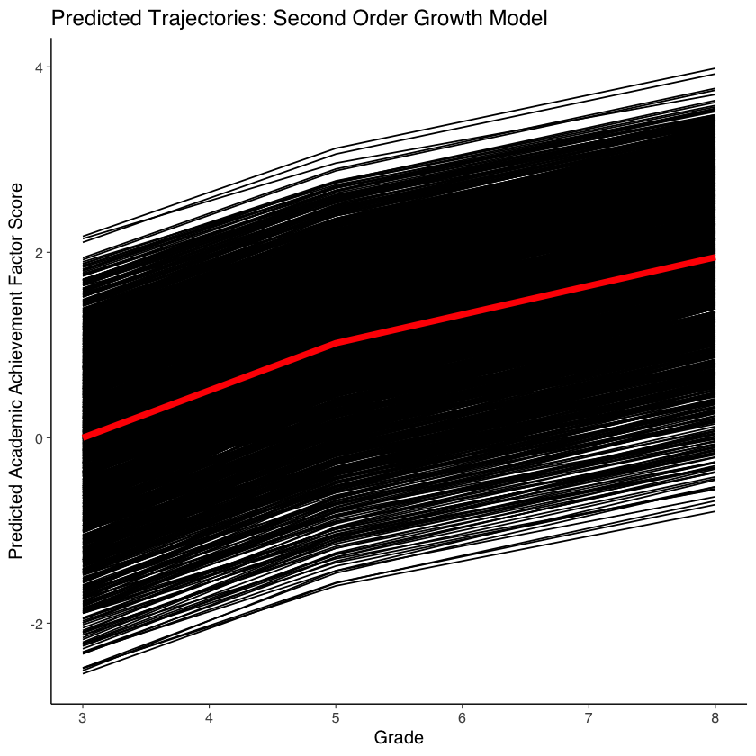
36.6. Conclusione#
Utilizzando più indicatori all’interno del framework di analisi dei fattori longitudinali, possiamo descrivere il cambiamento con maggiore precisione. Questo perché siamo in grado di filtrare il rumore di misura utilizzando un modello di misura multivariato. In questo modo, possiamo espandere le possibilità di indagine e studio delle differenze interindividuali nel cambiamento intra-individuale.