35. Modelli di crescita latenti bivariati#
I ricercatori spesso studiano più costrutti nel tempo per comprendere il loro sviluppo congiunto e le correlazioni tra di loro. Esistono diversi modelli statistici per studiare il cambiamento in più entità contemporaneamente. In questo capitolo ne copriamo due: il modello di crescita multivariato (MGM), che esamina le interrelazioni tra due processi di crescita distinti, e il modello di crescita con covariata variabile nel tempo (TVC), che stima l’effetto di una variabile che cambia nel tempo sui punteggi mentre modella contemporaneamente il cambiamento in quei punteggi con un modello di crescita. Questi modelli sono comuni nella ricerca sullo sviluppo e rispondono a domande specifiche riguardo le associazioni tra entità che cambiano simultaneamente e tra i cambiamenti per individui correlati.
Carichiamo i pacchetti necessari.
Questo tutorial mostra come adattare modelli di crescita lineare multivariati (bivariati) nel framework SEM in R. I dati sono tratti dal Capitolo 8 Grimm et al. [GRE16]. In particolare, utilizzando il set di dati NLSY-CYA, esaminiamo come le differenze individuali nella variazione del rendimento in matematica dei bambini durante la scuola siano correlate alle differenze individuali nella variazione dell’iperattività dei bambini (valutata dagli insegnanti). Iniziamo a leggere i dati.
# set filepath for data file
filepath <- "https://raw.githubusercontent.com/LRI-2/Data/main/GrowthModeling/nlsy_math_hyp_long_R.dat"
# read in the text data file using the url() function
dat <- read.table(
  file = url(filepath),
  na.strings = "."
) # indicates the missing data designator
# copy data with new name
nlsy_math_hyp_long <- dat

# Add names the columns of the data set
names(nlsy_math_hyp_long) <- c(
  "id", "female", "lb_wght", "anti_k1",
  "math", "comp", "rec", "bpi", "as", "anx", "hd",
  "hyp", "dp", "wd",
  "grade", "occ", "age", "men", "spring", "anti"
)

# reducing to variables of interest
nlsy_math_hyp_long <- nlsy_math_hyp_long[, c("id", "grade", "math", "hyp")]

# view the first few observations in the data set
head(nlsy_math_hyp_long, 10)
| id | grade | math | hyp | |
|---|---|---|---|---|
| <int> | <int> | <int> | <int> | |
| 1 | 201 | 3 | 38 | 0 |
| 2 | 201 | 5 | 55 | 0 |
| 3 | 303 | 2 | 26 | 1 |
| 4 | 303 | 5 | 33 | 1 |
| 5 | 2702 | 2 | 56 | 2 |
| 6 | 2702 | 4 | 58 | 3 |
| 7 | 2702 | 8 | 80 | 3 |
| 8 | 4303 | 3 | 41 | 1 |
| 9 | 4303 | 4 | 58 | 1 |
| 10 | 5002 | 4 | 46 | 3 |
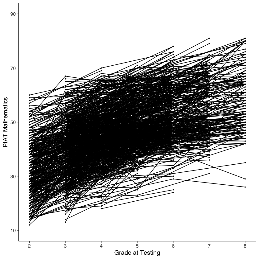
Il nostro interesse specifico è il cambiamento intra-individuale nelle misure ripetute di matematica e iperattività durante il periodo scolastico (grade).
# intraindividual change trajetories
ggplot(
  data = nlsy_math_hyp_long, # data set
  aes(x = grade, y = math, group = id)
) + # setting variables
  geom_point(size = .5) + # adding points to plot
  geom_line() + # adding lines to plot
  # setting the x-axis with breaks and labels
  scale_x_continuous(
    limits = c(2, 8),
    breaks = c(2, 3, 4, 5, 6, 7, 8),
    name = "Grade at Testing"
  ) +
  # setting the y-axis with limits breaks and labels
  scale_y_continuous(
    limits = c(10, 90),
    breaks = c(10, 30, 50, 70, 90),
    name = "PIAT Mathematics"
  )
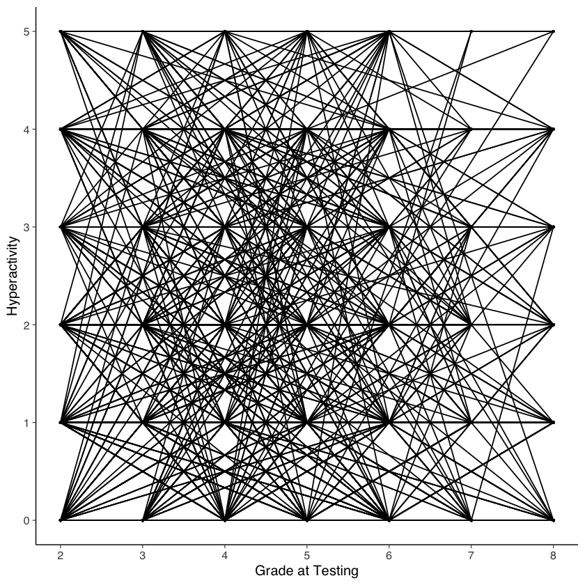
Esaminiamo i punteggi di iperattività in funzione di grade.
# intraindividual change trajetories
ggplot(
  data = nlsy_math_hyp_long, # data set
  aes(x = grade, y = hyp, group = id)
) + # setting variables
  geom_point(size = .5) + # adding points to plot
  geom_line() + # adding lines to plot
  # setting the x-axis with breaks and labels
  scale_x_continuous(
    limits = c(2, 8),
    breaks = c(2, 3, 4, 5, 6, 7, 8),
    name = "Grade at Testing"
  ) +
  # setting the y-axis with limits breaks and labels
  scale_y_continuous(
    limits = c(0, 5),
    breaks = c(0, 1, 2, 3, 4, 5),
    name = "Hyperactivity"
  )
Warning message:
“Removed 51 rows containing missing values (`geom_point()`).”
Warning message:
“Removed 44 rows containing missing values (`geom_line()`).”
Per semplicità, leggiamo i dati in formato long da file.
# set filepath for data file
filepath <- "https://raw.githubusercontent.com/LRI-2/Data/main/GrowthModeling/nlsy_math_hyp_wide_R.dat"
# read in the text data file using the url() function
dat <- read.table(
  file = url(filepath),
  na.strings = "."
) # indicates the missing data designator
# copy data with new name
nlsy_math_hyp_wide <- dat

# Add names the columns of the data set
# Give the variable names
names(nlsy_math_hyp_wide) <- c(
  "id", "female", "lb_wght", "anti_k1",
  "math2", "math3", "math4", "math5", "math6", "math7", "math8",
  "comp2", "comp3", "comp4", "comp5", "comp6", "comp7", "comp8",
  "rec2", "rec3", "rec4", "rec5", "rec6", "rec7", "rec8",
  "bpi2", "bpi3", "bpi4", "bpi5", "bpi6", "bpi7", "bpi8",
  "asl2", "asl3", "asl4", "asl5", "asl6", "asl7", "asl8",
  "ax2", "ax3", "ax4", "ax5", "ax6", "ax7", "ax8",
  "hds2", "hds3", "hds4", "hds5", "hds6", "hds7", "hds8",
  "hyp2", "hyp3", "hyp4", "hyp5", "hyp6", "hyp7", "hyp8",
  "dpn2", "dpn3", "dpn4", "dpn5", "dpn6", "dpn7", "dpn8",
  "wdn2", "wdn3", "wdn4", "wdn5", "wdn6", "wdn7", "wdn8",
  "age2", "age3", "age4", "age5", "age6", "age7", "age8",
  "men2", "men3", "men4", "men5", "men6", "men7", "men8",
  "spring2", "spring3", "spring4", "spring5", "spring6", "spring7", "spring8",
  "anti2", "anti3", "anti4", "anti5", "anti6", "anti7", "anti8"
)

# reducing to variables of interest
nlsy_multi_wide <- nlsy_math_hyp_wide[, c(
  "id",
  "math2", "math3", "math4", "math5", "math6", "math7", "math8",
  "hyp2", "hyp3", "hyp4", "hyp5", "hyp6", "hyp7", "hyp8"
)]

# view the first few observations in the data set
head(nlsy_multi_wide, 10)
| id | math2 | math3 | math4 | math5 | math6 | math7 | math8 | hyp2 | hyp3 | hyp4 | hyp5 | hyp6 | hyp7 | hyp8 | |
|---|---|---|---|---|---|---|---|---|---|---|---|---|---|---|---|
| <int> | <int> | <int> | <int> | <int> | <int> | <int> | <int> | <int> | <int> | <int> | <int> | <int> | <int> | <int> | |
| 1 | 201 | NA | 38 | NA | 55 | NA | NA | NA | NA | 0 | NA | 0 | NA | NA | NA |
| 2 | 303 | 26 | NA | NA | 33 | NA | NA | NA | 1 | NA | NA | 1 | NA | NA | NA |
| 3 | 2702 | 56 | NA | 58 | NA | NA | NA | 80 | 2 | NA | 3 | NA | NA | NA | 3 |
| 4 | 4303 | NA | 41 | 58 | NA | NA | NA | NA | NA | 1 | 1 | NA | NA | NA | NA |
| 5 | 5002 | NA | NA | 46 | NA | 54 | NA | 66 | NA | NA | 3 | NA | 2 | NA | 3 |
| 6 | 5005 | 35 | NA | 50 | NA | 60 | NA | 59 | 0 | NA | 3 | NA | 0 | NA | 1 |
| 7 | 5701 | NA | 62 | 61 | NA | NA | NA | NA | NA | 4 | 3 | NA | NA | NA | NA |
| 8 | 6102 | NA | NA | 55 | 67 | NA | 81 | NA | NA | NA | 2 | 0 | NA | 0 | NA |
| 9 | 6801 | NA | 54 | NA | 62 | NA | 66 | NA | NA | 0 | NA | 1 | NA | 1 | NA |
| 10 | 6802 | NA | 55 | NA | 66 | NA | 68 | NA | NA | 0 | NA | 0 | NA | 0 | NA |
Per l’implementazione SEM, utilizziamo i punteggi di rendimento in matematica e iperattività e le covariate invarianti nel tempo dai dati Wide. Specifichiamo un modello di crescita lineare bivariato usando la sintassi lavaan.
# writing out linear growth model in full SEM way
bivariate_lavaan_model <- "
  # latent variable definitions
      #intercept for math
      eta_1 =~ 1*math2
      eta_1 =~ 1*math3
      eta_1 =~ 1*math4
      eta_1 =~ 1*math5
      eta_1 =~ 1*math6
      eta_1 =~ 1*math7
      eta_1 =~ 1*math8

      #linear slope for math
      eta_2 =~ 0*math2
      eta_2 =~ 1*math3
      eta_2 =~ 2*math4
      eta_2 =~ 3*math5
      eta_2 =~ 4*math6
      eta_2 =~ 5*math7
      eta_2 =~ 6*math8

      #intercept for hyp
      eta_3 =~ 1*hyp2
      eta_3 =~ 1*hyp3
      eta_3 =~ 1*hyp4
      eta_3 =~ 1*hyp5
      eta_3 =~ 1*hyp6
      eta_3 =~ 1*hyp7
      eta_3 =~ 1*hyp8

      #linear slope for hyp
      eta_4 =~ 0*hyp2
      eta_4 =~ 1*hyp3
      eta_4 =~ 2*hyp4
      eta_4 =~ 3*hyp5
      eta_4 =~ 4*hyp6
      eta_4 =~ 5*hyp7
      eta_4 =~ 6*hyp8

  # factor variances
      eta_1 ~~ eta_1
      eta_2 ~~ eta_2
      eta_3 ~~ eta_3
      eta_4 ~~ eta_4

  # covariances among factors
      eta_1 ~~ eta_2 + eta_3 + eta_4
      eta_2 ~~ eta_3 + eta_4
      eta_3 ~~ eta_4

  # factor means
      eta_1 ~ start(35)*1
      eta_2 ~ start(4)*1
      eta_3 ~ start(2)*1
      eta_4 ~ start(.1)*1

  # manifest variances for math (made equivalent by naming theta1)
      math2 ~~ theta1*math2
      math3 ~~ theta1*math3
      math4 ~~ theta1*math4
      math5 ~~ theta1*math5
      math6 ~~ theta1*math6
      math7 ~~ theta1*math7
      math8 ~~ theta1*math8

  # manifest variances for hyp (made equivalent by naming theta2)
      hyp2 ~~ theta2*hyp2
      hyp3 ~~ theta2*hyp3
      hyp4 ~~ theta2*hyp4
      hyp5 ~~ theta2*hyp5
      hyp6 ~~ theta2*hyp6
      hyp7 ~~ theta2*hyp7
      hyp8 ~~ theta2*hyp8

  # residual covariances (made equivalent by naming theta12)
      math2 ~~ theta12*hyp2
      math3 ~~ theta12*hyp3
      math4 ~~ theta12*hyp4
      math5 ~~ theta12*hyp5
      math6 ~~ theta12*hyp6
      math7 ~~ theta12*hyp7
      math8 ~~ theta12*hyp8

  # manifest means for math (fixed at zero)
      math2 ~ 0*1
      math3 ~ 0*1
      math4 ~ 0*1
      math5 ~ 0*1
      math6 ~ 0*1
      math7 ~ 0*1
      math8 ~ 0*1

  # manifest means for hyp (fixed at zero)
      hyp2 ~ 0*1
      hyp3 ~ 0*1
      hyp4 ~ 0*1
      hyp5 ~ 0*1
      hyp6 ~ 0*1
      hyp7 ~ 0*1
      hyp8 ~ 0*1
" # end of model definition
Adattiamo il modello ai dati.
bivariate_lavaan_fit <- sem(bivariate_lavaan_model,
  data = nlsy_multi_wide,
  meanstructure = TRUE,
  estimator = "ML",
  missing = "fiml"
)
Warning message in lav_data_full(data = data, group = group, cluster = cluster, :
“lavaan WARNING: some cases are empty and will be ignored:
  741”
Warning message in lav_data_full(data = data, group = group, cluster = cluster, :
“lavaan WARNING:
    due to missing values, some pairwise combinations have less than
    10% coverage; use lavInspect(fit, "coverage") to investigate.”
Warning message in lav_mvnorm_missing_h1_estimate_moments(Y = X[[g]], wt = WT[[g]], :
“lavaan WARNING:
    Maximum number of iterations reached when computing the sample
    moments using EM; use the em.h1.iter.max= argument to increase the
    number of iterations”
Esaminiamo i risultati.
out = summary(bivariate_lavaan_fit, fit.measures = TRUE)
print(out)
lavaan 0.6.15 ended normally after 67 iterations

  Estimator                                         ML
  Optimization method                           NLMINB
  Number of model parameters                        35
  Number of equality constraints                    18

                                                  Used       Total
  Number of observations                           932         933
  Number of missing patterns                        96

Model Test User Model:

  Test statistic                               318.885
  Degrees of freedom                               102
  P-value (Chi-square)                           0.000

Model Test Baseline Model:

  Test statistic                              1532.041
  Degrees of freedom                                91
  P-value                                        0.000

User Model versus Baseline Model:

  Comparative Fit Index (CFI)                    0.849
  Tucker-Lewis Index (TLI)                       0.866

  Robust Comparative Fit Index (CFI)             1.000
  Robust Tucker-Lewis Index (TLI)               -6.557

Loglikelihood and Information Criteria:

  Loglikelihood user model (H0)             -11790.476
  Loglikelihood unrestricted model (H1)     -11631.033

  Akaike (AIC)                               23614.951
  Bayesian (BIC)                             23697.186
  Sample-size adjusted Bayesian (SABIC)      23643.196

Root Mean Square Error of Approximation:

  RMSEA                                          0.048
  90 Percent confidence interval - lower         0.042
  90 Percent confidence interval - upper         0.054
  P-value H_0: RMSEA <= 0.050                    0.724
  P-value H_0: RMSEA >= 0.080                    0.000

  Robust RMSEA                                   0.000
  90 Percent confidence interval - lower         0.000
  90 Percent confidence interval - upper         0.000
  P-value H_0: Robust RMSEA <= 0.050             1.000
  P-value H_0: Robust RMSEA >= 0.080             0.000

Standardized Root Mean Square Residual:

  SRMR                                           0.097

Parameter Estimates:

  Standard errors                             Standard
  Information                                 Observed
  Observed information based on                Hessian

Latent Variables:
                   Estimate  Std.Err  z-value  P(>|z|)
  eta_1 =~
    math2             1.000
    math3             1.000
    math4             1.000
    math5             1.000
    math6             1.000
    math7             1.000
    math8             1.000
  eta_2 =~
    math2             0.000
    math3             1.000
    math4             2.000
    math5             3.000
    math6             4.000
    math7             5.000
    math8             6.000
  eta_3 =~
    hyp2              1.000
    hyp3              1.000
    hyp4              1.000
    hyp5              1.000
    hyp6              1.000
    hyp7              1.000
    hyp8              1.000
  eta_4 =~
    hyp2              0.000
    hyp3              1.000
    hyp4              2.000
    hyp5              3.000
    hyp6              4.000
    hyp7              5.000
    hyp8              6.000

Covariances:
                   Estimate  Std.Err  z-value  P(>|z|)
  eta_1 ~~
    eta_2            -0.204    1.154   -0.176    0.860
    eta_3            -2.979    0.673   -4.426    0.000
    eta_4             0.107    0.164    0.654    0.513
  eta_2 ~~
    eta_3             0.098    0.161    0.608    0.543
    eta_4            -0.040    0.038   -1.061    0.289
  eta_3 ~~
    eta_4            -0.020    0.031   -0.644    0.520
 .math2 ~~
   .hyp2    (th12)   -0.011    0.233   -0.046    0.963
 .math3 ~~
   .hyp3    (th12)   -0.011    0.233   -0.046    0.963
 .math4 ~~
   .hyp4    (th12)   -0.011    0.233   -0.046    0.963
 .math5 ~~
   .hyp5    (th12)   -0.011    0.233   -0.046    0.963
 .math6 ~~
   .hyp6    (th12)   -0.011    0.233   -0.046    0.963
 .math7 ~~
   .hyp7    (th12)   -0.011    0.233   -0.046    0.963
 .math8 ~~
   .hyp8    (th12)   -0.011    0.233   -0.046    0.963

Intercepts:
                   Estimate  Std.Err  z-value  P(>|z|)
    eta_1            35.259    0.356   99.178    0.000
    eta_2             4.343    0.088   49.139    0.000
    eta_3             1.903    0.058   32.702    0.000
    eta_4            -0.057    0.014   -3.950    0.000
   .math2             0.000
   .math3             0.000
   .math4             0.000
   .math5             0.000
   .math6             0.000
   .math7             0.000
   .math8             0.000
   .hyp2              0.000
   .hyp3              0.000
   .hyp4              0.000
   .hyp5              0.000
   .hyp6              0.000
   .hyp7              0.000
   .hyp8              0.000

Variances:
                   Estimate  Std.Err  z-value  P(>|z|)
    eta_1            64.711    5.664   11.424    0.000
    eta_2             0.752    0.329    2.282    0.023
    eta_3             1.542    0.156    9.908    0.000
    eta_4             0.005    0.009    0.539    0.590
   .math2   (tht1)   36.126    1.863   19.390    0.000
   .math3   (tht1)   36.126    1.863   19.390    0.000
   .math4   (tht1)   36.126    1.863   19.390    0.000
   .math5   (tht1)   36.126    1.863   19.390    0.000
   .math6   (tht1)   36.126    1.863   19.390    0.000
   .math7   (tht1)   36.126    1.863   19.390    0.000
   .math8   (tht1)   36.126    1.863   19.390    0.000
   .hyp2    (tht2)    1.104    0.057   19.404    0.000
   .hyp3    (tht2)    1.104    0.057   19.404    0.000
   .hyp4    (tht2)    1.104    0.057   19.404    0.000
   .hyp5    (tht2)    1.104    0.057   19.404    0.000
   .hyp6    (tht2)    1.104    0.057   19.404    0.000
   .hyp7    (tht2)    1.104    0.057   19.404    0.000
   .hyp8    (tht2)    1.104    0.057   19.404    0.000
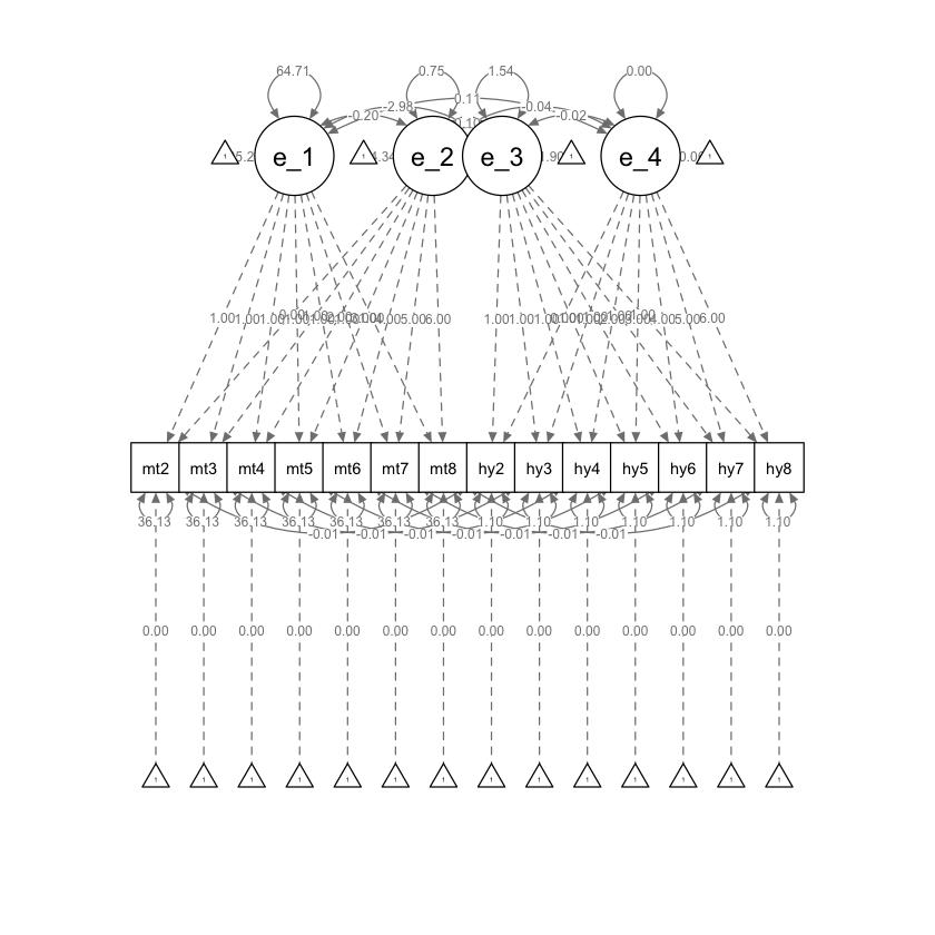
Il parametro principale di interesse, la covarianza pendenza-pendenza eta_3 ~~eta_4, non è significativamente diverso da zero.
Generiamo un diagramma di percorso.
semPaths(bivariate_lavaan_fit, what = "path", whatLabels = "par")
35.1. Conclusione#
Questo tutorial ha presentato come il modello di crescita multivariato possa essere utilizzato per esaminare le interrelazioni nel cambiamento - in particolare la correlazione between-person tra le pendenze.