32. Il tempo su una metrica continua#
Quando si cerca di comprendere il cambiamento all’interno della persona, una prima decisione importante è quella di scegliere una scala temporale appropriata per monitorare il cambiamento. Ad esempio, nell’esempio illustrativo discusso nel capitolo precedente, abbiamo scelto il grado scolastico come scala temporale e abbiamo organizzato le osservazioni attorno a questa metrica. Tuttavia, questa non è l’unica metrica del tempo possibile per questi dati. Altre metriche potenzialmente significative includono l’età e l’occasione di misurazione. Esistono metriche del tempo che rappresentano intervalli di tempo discreti, come l’occasione di misurazione o il grado scolastico, dove la metrica assume valori discreti comuni ai partecipanti. Ma non tutti i partecipanti devono essere valutati in ogni occasione di misurazione. Esistono anche metriche del tempo più continue, come l’età, dove i valori non sono comuni a più partecipanti. La stessa metrica può essere utilizzata in modo discreto o continuo. Ad esempio, l’età potrebbe essere arrotondata all’anno più vicino e il grado scolastico potrebbe essere misurato con precisione come anno scolastico più i giorni dall’inizio dell’anno. In questo capitolo discutiamo tecniche per adattare modelli di crescita con una metrica del tempo continua.
32.1. Una applicazione concreta#
L’approccio della finestra temporale è un metodo potenziale per analizzare dati con occasioni di misurazione individualmente variabili. In sostanza, l’approccio della finestra temporale mira ad approssimare la metrica del tempo individualmente variabile su una scala discreta. Ad esempio, ciò può essere ottenuto arrotondando il tempo/l’età al mezzo o al quarto d’anno più vicino.
Questo metodo è ovviamente ancora un’approssimazione del tempo. Si può ottenere maggiore precisione utilizzando finestre più piccole, ma se la matrice dei dati diventa troppo sparsa, la stima diventa difficile.
In questo esempio, le finestre temporali sono definite come semestri. Quindi, prendiamo i nostri dati in formato long, arrotondiamo l’età al semestre più vicino e convertiamo i dati in formato wide per l’utilizzo nel framework SEM.
Per questo esempio considereremo i dati di presrtazione matematica dal data set NLSY-CYA Long Data [si veda Grimm et al. [GRE16]]. Iniziamo a leggere i dati.
#set filepath for data file
filepath <- "https://raw.githubusercontent.com/LRI-2/Data/main/GrowthModeling/nlsy_math_long_R.dat"
#read in the text data file using the url() function
dat <- read.table(file=url(filepath),
                  na.strings = ".")  #indicates the missing data designator
#copy data with new name
nlsy_math_long <- dat

#Add names the columns of the data set
names(nlsy_math_long) = c('id'     , 'female', 'lb_wght',
                          'anti_k1', 'math'  , 'grade'  ,
                          'occ'    , 'age'   , 'men'    ,
                          'spring' , 'anti')

#subset to the variables of interest
nlsy_math_long <- nlsy_math_long[ ,c("id", "math", "grade", "age")]
#view the first few observations in the data set
head(nlsy_math_long, 10)
| id | math | grade | age | |
|---|---|---|---|---|
| <int> | <int> | <int> | <int> | |
| 1 | 201 | 38 | 3 | 111 |
| 2 | 201 | 55 | 5 | 135 |
| 3 | 303 | 26 | 2 | 121 |
| 4 | 303 | 33 | 5 | 145 |
| 5 | 2702 | 56 | 2 | 100 |
| 6 | 2702 | 58 | 4 | 125 |
| 7 | 2702 | 80 | 8 | 173 |
| 8 | 4303 | 41 | 3 | 115 |
| 9 | 4303 | 58 | 4 | 135 |
| 10 | 5002 | 46 | 4 | 117 |
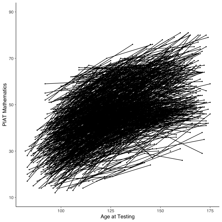
#intraindividual change trajetories
ggplot(data=nlsy_math_long,                    #data set
       aes(x = age, y = math, group = id)) + #setting variables
  geom_point(size=.5) + #adding points to plot
  geom_line() +  #adding lines to plot
  #setting the x-axis with breaks and labels
  scale_x_continuous(#limits=c(2,8),
                     #breaks = c(2,3,4,5,6,7,8),
                     name = "Age at Testing") +
  #setting the y-axis with limits breaks and labels
  scale_y_continuous(limits=c(10,90),
                     breaks = c(10,30,50,70,90),
                     name = "PIAT Mathematics")
Implementiamo il metodo della finestra temporale e ricodifichiamo i dati in formato wide.
# creating new age variable scaled in years
nlsy_math_long$ageyr <- (nlsy_math_long$age / 12)
head(nlsy_math_long)
| id | math | grade | age | ageyr | |
|---|---|---|---|---|---|
| <int> | <int> | <int> | <int> | <dbl> | |
| 1 | 201 | 38 | 3 | 111 | 9.250000 |
| 2 | 201 | 55 | 5 | 135 | 11.250000 |
| 3 | 303 | 26 | 2 | 121 | 10.083333 |
| 4 | 303 | 33 | 5 | 145 | 12.083333 |
| 5 | 2702 | 56 | 2 | 100 | 8.333333 |
| 6 | 2702 | 58 | 4 | 125 | 10.416667 |
# rounding to nearest half-year
# multiplied by 10 to remove decimal for easy conversion to wide
nlsy_math_long$agewindow <- plyr::round_any(nlsy_math_long$ageyr * 10, 5)
head(nlsy_math_long)
| id | math | grade | age | ageyr | agewindow | |
|---|---|---|---|---|---|---|
| <int> | <int> | <int> | <int> | <dbl> | <dbl> | |
| 1 | 201 | 38 | 3 | 111 | 9.250000 | 90 |
| 2 | 201 | 55 | 5 | 135 | 11.250000 | 110 |
| 3 | 303 | 26 | 2 | 121 | 10.083333 | 100 |
| 4 | 303 | 33 | 5 | 145 | 12.083333 | 120 |
| 5 | 2702 | 56 | 2 | 100 | 8.333333 | 85 |
| 6 | 2702 | 58 | 4 | 125 | 10.416667 | 105 |
# reshaping long to wide (just variables of interest)
nlsy_math_wide <- reshape(
  data = nlsy_math_long[, c("id", "math", "agewindow")],
  timevar = c("agewindow"),
  idvar = c("id"),
  v.names = c("math"),
  direction = "wide", sep = ""
)

# reordering columns for easy viewing
nlsy_math_wide <- nlsy_math_wide[, c(
  "id", "math70", "math75", "math80", "math85", "math90", "math95", "math100", "math105", "math110", "math115", "math120", "math125", "math130", "math135", "math140", "math145"
)]
# looking at the data
head(nlsy_math_wide)
| id | math70 | math75 | math80 | math85 | math90 | math95 | math100 | math105 | math110 | math115 | math120 | math125 | math130 | math135 | math140 | math145 | |
|---|---|---|---|---|---|---|---|---|---|---|---|---|---|---|---|---|---|
| <int> | <int> | <int> | <int> | <int> | <int> | <int> | <int> | <int> | <int> | <int> | <int> | <int> | <int> | <int> | <int> | <int> | |
| 1 | 201 | NA | NA | NA | NA | 38 | NA | NA | NA | 55 | NA | NA | NA | NA | NA | NA | NA |
| 3 | 303 | NA | NA | NA | NA | NA | NA | 26 | NA | NA | NA | 33 | NA | NA | NA | NA | NA |
| 5 | 2702 | NA | NA | NA | 56 | NA | NA | NA | 58 | NA | NA | NA | NA | NA | NA | NA | 80 |
| 8 | 4303 | NA | NA | NA | NA | NA | 41 | NA | NA | 58 | NA | NA | NA | NA | NA | NA | NA |
| 10 | 5002 | NA | NA | NA | NA | NA | NA | 46 | NA | NA | NA | 54 | NA | NA | NA | 66 | NA |
| 13 | 5005 | NA | NA | 35 | NA | NA | 50 | NA | NA | NA | 60 | NA | NA | NA | 59 | NA | NA |
Specifichiamo il modello SEM.
#writing out linear growth model in full SEM way
lg_math_age_lavaan_model <- '
  # latent variable definitions
      #intercept (note intercept is a reserved term)
      eta_1 =~  1*math70 +
                1*math75 +
                1*math80 +
                1*math85 +
                1*math90 +
                1*math95 +
                1*math100 +
                1*math105 +
                1*math110 +
                1*math115 +
                1*math120 +
                1*math125 +
                1*math130 +
                1*math135 +
                1*math140 +
                1*math145

      #linear slope (note intercept is a reserved term)
      eta_2 =~ -1*math70 +
               -0.5*math75 +
                0*math80 +
                0.5*math85 +
                1*math90 +
                1.5*math95 +
                2*math100 +
                2.5*math105 +
                3*math110 +
                3.5*math115 +
                4*math120 +
                4.5*math125 +
                5*math130 +
                5.5*math135 +
                6*math140 +
                6.5*math145

  # factor variances
      eta_1 ~~ start(65)*eta_1
      eta_2 ~~ start(.75)*eta_2

  # covariances among factors
      eta_1 ~~ start(1.2)*eta_2

  # manifest variances (made equivalent by naming theta)
      math70 ~~ start(35)*theta*math70
      math75 ~~ theta*math75
      math80 ~~ theta*math80
      math85 ~~ theta*math85
      math90 ~~ theta*math90
      math95 ~~ theta*math95
      math100 ~~ theta*math100
      math105 ~~ theta*math105
      math110 ~~ theta*math110
      math115 ~~ theta*math115
      math120 ~~ theta*math120
      math125 ~~ theta*math125
      math130 ~~ theta*math130
      math135 ~~ theta*math135
      math140 ~~ theta*math140
      math145 ~~ theta*math145

  # manifest means (fixed at zero)
      math70 ~ 0*1
      math75 ~ 0*1
      math80 ~ 0*1
      math85 ~ 0*1
      math90 ~ 0*1
      math95 ~ 0*1
      math100 ~ 0*1
      math105 ~ 0*1
      math110 ~ 0*1
      math115 ~ 0*1
      math120 ~ 0*1
      math125 ~ 0*1
      math130 ~ 0*1
      math135 ~ 0*1
      math140 ~ 0*1
      math145 ~ 0*1

  # factor means (estimated freely)
      eta_1 ~ start(35)*1
      eta_2 ~ start(4)*1
' #end of model definition
Adattiamo il modello ai dati.
#estimating the model using sem() function
lg_math_age_lavaan_fit <- sem(lg_math_age_lavaan_model,
  data = nlsy_math_wide,
  meanstructure = TRUE,
  estimator = "ML",
  missing = "fiml"
)
Warning message in lav_data_full(data = data, group = group, cluster = cluster, :
“lavaan WARNING:
    due to missing values, some pairwise combinations have 0%
    coverage; use lavInspect(fit, "coverage") to investigate.”
Warning message in lav_mvnorm_missing_h1_estimate_moments(Y = X[[g]], wt = WT[[g]], :
“lavaan WARNING:
    Maximum number of iterations reached when computing the sample
    moments using EM; use the em.h1.iter.max= argument to increase the
    number of iterations”
Esaminiamo la soluzione.
summary(lg_math_age_lavaan_fit, fit.measures = TRUE) |>
    print()
Warning message in pchisq(X2, df = df, ncp = ncp):
“NaNs produced”
Warning message in pchisq(X2, df = df, ncp = ncp):
“NaNs produced”
lavaan 0.6.15 ended normally after 27 iterations

  Estimator                                         ML
  Optimization method                           NLMINB
  Number of model parameters                        21
  Number of equality constraints                    15

  Number of observations                           932
  Number of missing patterns                       139

Model Test User Model:

  Test statistic                               295.028
  Degrees of freedom                               146
  P-value (Chi-square)                           0.000

Model Test Baseline Model:

  Test statistic                              1053.342
  Degrees of freedom                               120
  P-value                                        0.000

User Model versus Baseline Model:

  Comparative Fit Index (CFI)                    0.840
  Tucker-Lewis Index (TLI)                       0.869

  Robust Comparative Fit Index (CFI)             0.003
  Robust Tucker-Lewis Index (TLI)                0.181

Loglikelihood and Information Criteria:

  Loglikelihood user model (H0)              -7928.559
  Loglikelihood unrestricted model (H1)      -7781.045

  Akaike (AIC)                               15869.117
  Bayesian (BIC)                             15898.141
  Sample-size adjusted Bayesian (SABIC)      15879.086

Root Mean Square Error of Approximation:

  RMSEA                                          0.033
  90 Percent confidence interval - lower         0.028
  90 Percent confidence interval - upper         0.039
  P-value H_0: RMSEA <= 0.050                    1.000
  P-value H_0: RMSEA >= 0.080                    0.000

  Robust RMSEA                                   4.193
  90 Percent confidence interval - lower         0.000
  90 Percent confidence interval - upper         0.000
  P-value H_0: Robust RMSEA <= 0.050               NaN
  P-value H_0: Robust RMSEA >= 0.080               NaN

Standardized Root Mean Square Residual:

  SRMR                                           0.314

Parameter Estimates:

  Standard errors                             Standard
  Information                                 Observed
  Observed information based on                Hessian

Latent Variables:
                   Estimate  Std.Err  z-value  P(>|z|)
  eta_1 =~
    math70            1.000
    math75            1.000
    math80            1.000
    math85            1.000
    math90            1.000
    math95            1.000
    math100           1.000
    math105           1.000
    math110           1.000
    math115           1.000
    math120           1.000
    math125           1.000
    math130           1.000
    math135           1.000
    math140           1.000
    math145           1.000
  eta_2 =~
    math70           -1.000
    math75           -0.500
    math80            0.000
    math85            0.500
    math90            1.000
    math95            1.500
    math100           2.000
    math105           2.500
    math110           3.000
    math115           3.500
    math120           4.000
    math125           4.500
    math130           5.000
    math135           5.500
    math140           6.000
    math145           6.500

Covariances:
                   Estimate  Std.Err  z-value  P(>|z|)
  eta_1 ~~
    eta_2             1.157    1.010    1.146    0.252

Intercepts:
                   Estimate  Std.Err  z-value  P(>|z|)
   .math70            0.000
   .math75            0.000
   .math80            0.000
   .math85            0.000
   .math90            0.000
   .math95            0.000
   .math100           0.000
   .math105           0.000
   .math110           0.000
   .math115           0.000
   .math120           0.000
   .math125           0.000
   .math130           0.000
   .math135           0.000
   .math140           0.000
   .math145           0.000
    eta_1            35.236    0.347  101.512    0.000
    eta_2             4.229    0.081   51.910    0.000

Variances:
                   Estimate  Std.Err  z-value  P(>|z|)
    eta_1            65.063    5.503   11.824    0.000
    eta_2             0.725    0.277    2.616    0.009
   .math70  (thet)   32.337    1.695   19.083    0.000
   .math75  (thet)   32.337    1.695   19.083    0.000
   .math80  (thet)   32.337    1.695   19.083    0.000
   .math85  (thet)   32.337    1.695   19.083    0.000
   .math90  (thet)   32.337    1.695   19.083    0.000
   .math95  (thet)   32.337    1.695   19.083    0.000
   .math100 (thet)   32.337    1.695   19.083    0.000
   .math105 (thet)   32.337    1.695   19.083    0.000
   .math110 (thet)   32.337    1.695   19.083    0.000
   .math115 (thet)   32.337    1.695   19.083    0.000
   .math120 (thet)   32.337    1.695   19.083    0.000
   .math125 (thet)   32.337    1.695   19.083    0.000
   .math130 (thet)   32.337    1.695   19.083    0.000
   .math135 (thet)   32.337    1.695   19.083    0.000
   .math140 (thet)   32.337    1.695   19.083    0.000
   .math145 (thet)   32.337    1.695   19.083    0.000
parameterEstimates(lg_math_age_lavaan_fit) |>
    print()
       lhs op     rhs label    est    se       z pvalue ci.lower ci.upper
1    eta_1 =~  math70        1.000 0.000      NA     NA    1.000    1.000
2    eta_1 =~  math75        1.000 0.000      NA     NA    1.000    1.000
3    eta_1 =~  math80        1.000 0.000      NA     NA    1.000    1.000
4    eta_1 =~  math85        1.000 0.000      NA     NA    1.000    1.000
5    eta_1 =~  math90        1.000 0.000      NA     NA    1.000    1.000
6    eta_1 =~  math95        1.000 0.000      NA     NA    1.000    1.000
7    eta_1 =~ math100        1.000 0.000      NA     NA    1.000    1.000
8    eta_1 =~ math105        1.000 0.000      NA     NA    1.000    1.000
9    eta_1 =~ math110        1.000 0.000      NA     NA    1.000    1.000
10   eta_1 =~ math115        1.000 0.000      NA     NA    1.000    1.000
11   eta_1 =~ math120        1.000 0.000      NA     NA    1.000    1.000
12   eta_1 =~ math125        1.000 0.000      NA     NA    1.000    1.000
13   eta_1 =~ math130        1.000 0.000      NA     NA    1.000    1.000
14   eta_1 =~ math135        1.000 0.000      NA     NA    1.000    1.000
15   eta_1 =~ math140        1.000 0.000      NA     NA    1.000    1.000
16   eta_1 =~ math145        1.000 0.000      NA     NA    1.000    1.000
17   eta_2 =~  math70       -1.000 0.000      NA     NA   -1.000   -1.000
18   eta_2 =~  math75       -0.500 0.000      NA     NA   -0.500   -0.500
19   eta_2 =~  math80        0.000 0.000      NA     NA    0.000    0.000
20   eta_2 =~  math85        0.500 0.000      NA     NA    0.500    0.500
21   eta_2 =~  math90        1.000 0.000      NA     NA    1.000    1.000
22   eta_2 =~  math95        1.500 0.000      NA     NA    1.500    1.500
23   eta_2 =~ math100        2.000 0.000      NA     NA    2.000    2.000
24   eta_2 =~ math105        2.500 0.000      NA     NA    2.500    2.500
25   eta_2 =~ math110        3.000 0.000      NA     NA    3.000    3.000
26   eta_2 =~ math115        3.500 0.000      NA     NA    3.500    3.500
27   eta_2 =~ math120        4.000 0.000      NA     NA    4.000    4.000
28   eta_2 =~ math125        4.500 0.000      NA     NA    4.500    4.500
29   eta_2 =~ math130        5.000 0.000      NA     NA    5.000    5.000
30   eta_2 =~ math135        5.500 0.000      NA     NA    5.500    5.500
31   eta_2 =~ math140        6.000 0.000      NA     NA    6.000    6.000
32   eta_2 =~ math145        6.500 0.000      NA     NA    6.500    6.500
33   eta_1 ~~   eta_1       65.063 5.503  11.824  0.000   54.278   75.849
34   eta_2 ~~   eta_2        0.725 0.277   2.616  0.009    0.182    1.268
35   eta_1 ~~   eta_2        1.157 1.010   1.146  0.252   -0.822    3.136
36  math70 ~~  math70 theta 32.337 1.695  19.083  0.000   29.016   35.658
37  math75 ~~  math75 theta 32.337 1.695  19.083  0.000   29.016   35.658
38  math80 ~~  math80 theta 32.337 1.695  19.083  0.000   29.016   35.658
39  math85 ~~  math85 theta 32.337 1.695  19.083  0.000   29.016   35.658
40  math90 ~~  math90 theta 32.337 1.695  19.083  0.000   29.016   35.658
41  math95 ~~  math95 theta 32.337 1.695  19.083  0.000   29.016   35.658
42 math100 ~~ math100 theta 32.337 1.695  19.083  0.000   29.016   35.658
43 math105 ~~ math105 theta 32.337 1.695  19.083  0.000   29.016   35.658
44 math110 ~~ math110 theta 32.337 1.695  19.083  0.000   29.016   35.658
45 math115 ~~ math115 theta 32.337 1.695  19.083  0.000   29.016   35.658
46 math120 ~~ math120 theta 32.337 1.695  19.083  0.000   29.016   35.658
47 math125 ~~ math125 theta 32.337 1.695  19.083  0.000   29.016   35.658
48 math130 ~~ math130 theta 32.337 1.695  19.083  0.000   29.016   35.658
49 math135 ~~ math135 theta 32.337 1.695  19.083  0.000   29.016   35.658
50 math140 ~~ math140 theta 32.337 1.695  19.083  0.000   29.016   35.658
51 math145 ~~ math145 theta 32.337 1.695  19.083  0.000   29.016   35.658
52  math70 ~1                0.000 0.000      NA     NA    0.000    0.000
53  math75 ~1                0.000 0.000      NA     NA    0.000    0.000
54  math80 ~1                0.000 0.000      NA     NA    0.000    0.000
55  math85 ~1                0.000 0.000      NA     NA    0.000    0.000
56  math90 ~1                0.000 0.000      NA     NA    0.000    0.000
57  math95 ~1                0.000 0.000      NA     NA    0.000    0.000
58 math100 ~1                0.000 0.000      NA     NA    0.000    0.000
59 math105 ~1                0.000 0.000      NA     NA    0.000    0.000
60 math110 ~1                0.000 0.000      NA     NA    0.000    0.000
61 math115 ~1                0.000 0.000      NA     NA    0.000    0.000
62 math120 ~1                0.000 0.000      NA     NA    0.000    0.000
63 math125 ~1                0.000 0.000      NA     NA    0.000    0.000
64 math130 ~1                0.000 0.000      NA     NA    0.000    0.000
65 math135 ~1                0.000 0.000      NA     NA    0.000    0.000
66 math140 ~1                0.000 0.000      NA     NA    0.000    0.000
67 math145 ~1                0.000 0.000      NA     NA    0.000    0.000
68   eta_1 ~1               35.236 0.347 101.512  0.000   34.556   35.917
69   eta_2 ~1                4.229 0.081  51.910  0.000    4.069    4.389
inspect(lg_math_age_lavaan_fit, what="est") |>
    print()
$lambda
        eta_1 eta_2
math70      1  -1.0
math75      1  -0.5
math80      1   0.0
math85      1   0.5
math90      1   1.0
math95      1   1.5
math100     1   2.0
math105     1   2.5
math110     1   3.0
math115     1   3.5
math120     1   4.0
math125     1   4.5
math130     1   5.0
math135     1   5.5
math140     1   6.0
math145     1   6.5

$theta
        math70 math75 math80 math85 math90 math95 mth100 mth105 mth110 mth115
math70  32.337
math75   0.000 32.337
math80   0.000  0.000 32.337
math85   0.000  0.000  0.000 32.337
math90   0.000  0.000  0.000  0.000 32.337
math95   0.000  0.000  0.000  0.000  0.000 32.337
math100  0.000  0.000  0.000  0.000  0.000  0.000 32.337
math105  0.000  0.000  0.000  0.000  0.000  0.000  0.000 32.337
math110  0.000  0.000  0.000  0.000  0.000  0.000  0.000  0.000 32.337
math115  0.000  0.000  0.000  0.000  0.000  0.000  0.000  0.000  0.000 32.337
math120  0.000  0.000  0.000  0.000  0.000  0.000  0.000  0.000  0.000  0.000
math125  0.000  0.000  0.000  0.000  0.000  0.000  0.000  0.000  0.000  0.000
math130  0.000  0.000  0.000  0.000  0.000  0.000  0.000  0.000  0.000  0.000
math135  0.000  0.000  0.000  0.000  0.000  0.000  0.000  0.000  0.000  0.000
math140  0.000  0.000  0.000  0.000  0.000  0.000  0.000  0.000  0.000  0.000
math145  0.000  0.000  0.000  0.000  0.000  0.000  0.000  0.000  0.000  0.000
        mth120 mth125 mth130 mth135 mth140 mth145
math70
math75
math80
math85
math90
math95
math100
math105
math110
math115
math120 32.337
math125  0.000 32.337
math130  0.000  0.000 32.337
math135  0.000  0.000  0.000 32.337
math140  0.000  0.000  0.000  0.000 32.337
math145  0.000  0.000  0.000  0.000  0.000 32.337

$psi
       eta_1  eta_2
eta_1 65.063
eta_2  1.157  0.725

$nu
        intrcp
math70       0
math75       0
math80       0
math85       0
math90       0
math95       0
math100      0
math105      0
math110      0
math115      0
math120      0
math125      0
math130      0
math135      0
math140      0
math145      0

$alpha
      intrcp
eta_1 35.236
eta_2  4.229
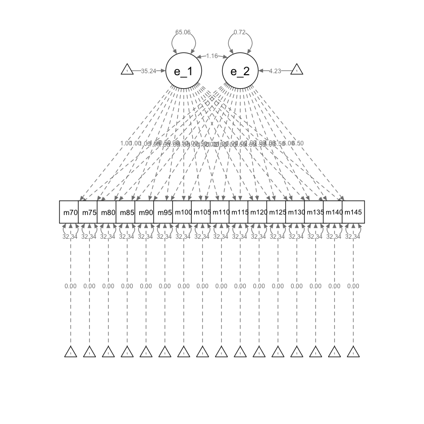
Creiamo un diagramma di percorso.
semPaths(lg_math_age_lavaan_fit,what = "path", whatLabels = "par")